SelfHosted Placement for Massively Parallel Processor Arrays MPPAs

Self-Hosted Placement for Massively Parallel Processor Arrays (MPPAs) Graeme Smecher, Steve Wilton, Guy Lemieux Thursday, December 10, 2009 FPT 2009

Landscape • Massively Parallel Processor Arrays – 2 D array of processors • Ambric: 336, Pico. Chip: 273, As. AP: 167, Tilera: 100 – Processor-to-processor communication • Placement (locality) matters – Tools/algorithms immature 2

Opportunity • MPPAs track Moore’s Law – Array size grows • E. g. Ambric: 336, Fermi: 512 • Opportunity for FPGA-like CAD? – Compiler-esque speed needed – Self-hosted parallel placement • M x N array of CPUs computes placement for M x N programs • Inherently scalable 3

Overview • • • Architecture Placement Problem Self-Hosted Placement Algorithm Experimental Results Conclusions 4

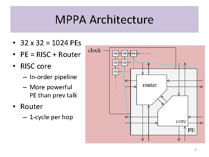
MPPA Architecture • 32 x 32 = 1024 PEs • PE = RISC + Router • RISC core – In-order pipeline – More powerful PE than prev talk • Router – 1 -cycle per hop 5

Overview • • • Architecture Placement Problem Self-Hosted Placement Algorithm Experimental Results Conclusions 7

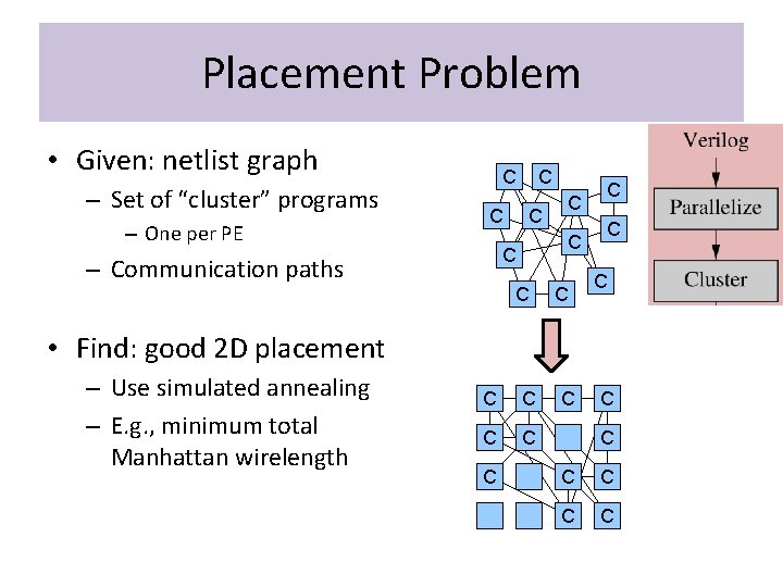
Placement Problem • Given: netlist graph – Set of “cluster” programs – One per PE C C C – Communication paths C C C • Find: good 2 D placement – Use simulated annealing – E. g. , minimum total Manhattan wirelength C C C C 8

Overview • • • Architecture Placement Problem Self-Hosted Placement Algorithm Experimental Results Conclusions 9

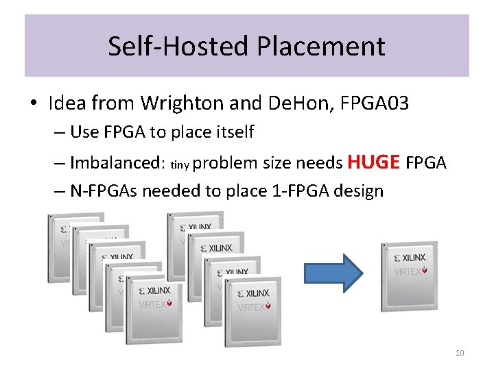
Self-Hosted Placement • Idea from Wrighton and De. Hon, FPGA 03 – Use FPGA to place itself – Imbalanced: tiny problem size needs HUGE FPGA – N-FPGAs needed to place 1 -FPGA design 10

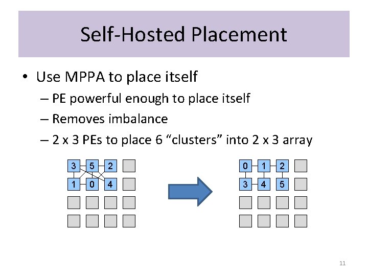
Self-Hosted Placement • Use MPPA to place itself – PE powerful enough to place itself – Removes imbalance – 2 x 3 PEs to place 6 “clusters” into 2 x 3 array C 3 C 5 C 2 C C 0 C 1 C 2 C C 1 C 0 4 C C C 3 C 4 5 C C C C C 11

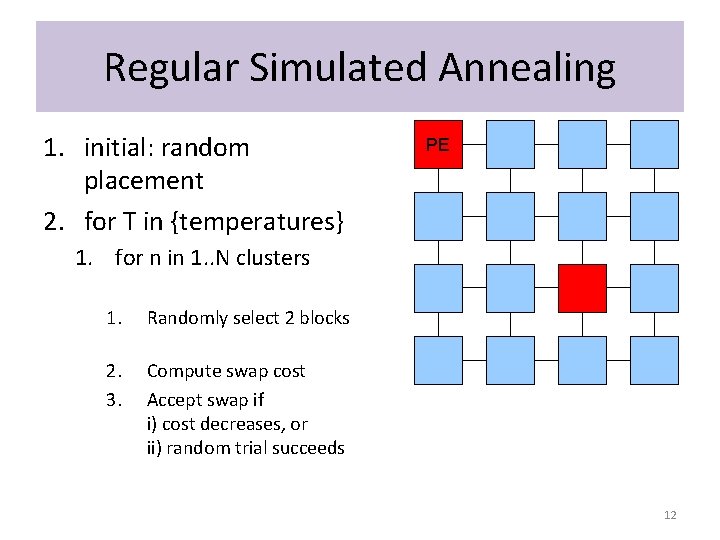
Regular Simulated Annealing 1. initial: random placement 2. for T in {temperatures} PE 1. for n in 1. . N clusters 1. Randomly select 2 blocks 2. 3. Compute swap cost Accept swap if i) cost decreases, or ii) random trial succeeds 12

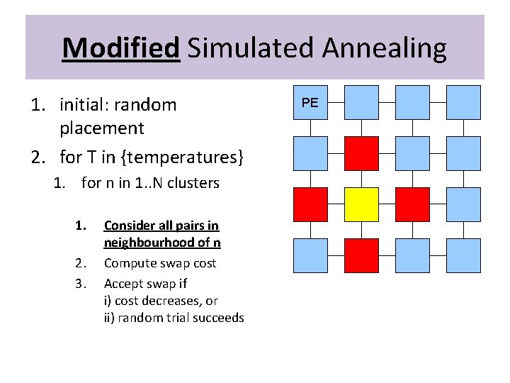
Modified Simulated Annealing 1. initial: random placement 2. for T in {temperatures} PE 1. for n in 1. . N clusters 1. 2. 3. Consider all pairs in neighbourhood of n Compute swap cost Accept swap if i) cost decreases, or ii) random trial succeeds 13

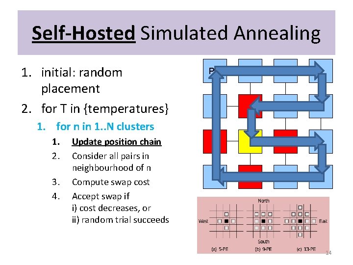
Self-Hosted Simulated Annealing 1. initial: random placement 2. for T in {temperatures} PE 1. for n in 1. . N clusters 1. 2. 3. 4. Update position chain Consider all pairs in neighbourhood of n Compute swap cost Accept swap if i) cost decreases, or ii) random trial succeeds 14

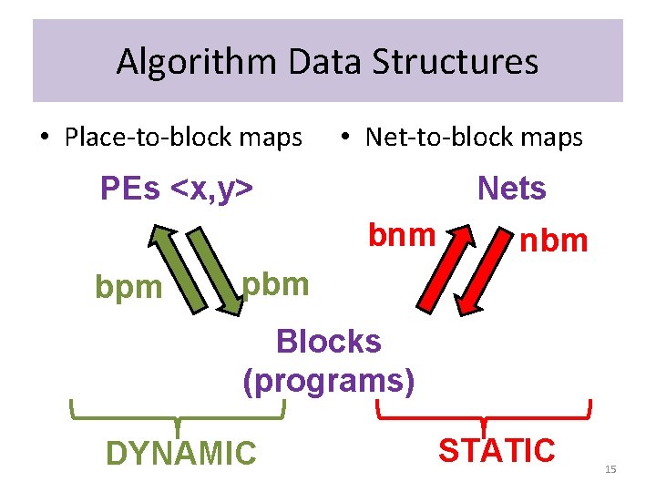
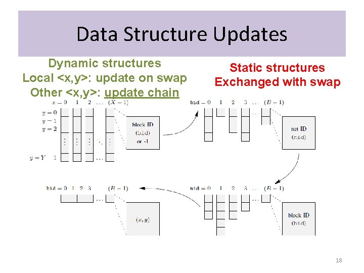
Algorithm Data Structures • Place-to-block maps • Net-to-block maps PEs <x, y> Nets bnm bpm nbm pbm Blocks (programs) DYNAMIC STATIC 15

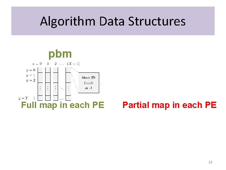
Algorithm Data Structures static pbm Full map in each PE bpm bnm Partial map in each PE nbm 16

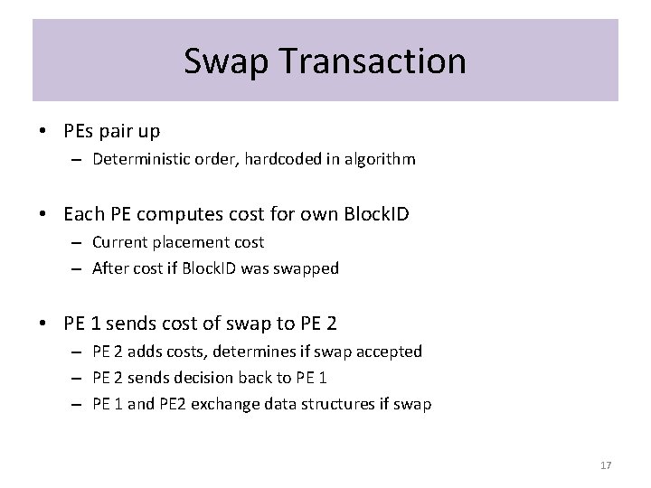
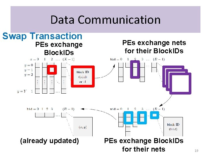
Swap Transaction • PEs pair up – Deterministic order, hardcoded in algorithm • Each PE computes cost for own Block. ID – Current placement cost – After cost if Block. ID was swapped • PE 1 sends cost of swap to PE 2 – PE 2 adds costs, determines if swap accepted – PE 2 sends decision back to PE 1 – PE 1 and PE 2 exchange data structures if swap 17

Data Structure Updates Dynamic structures Local <x, y>: update on swap Other <x, y>: update chain Static structures Exchanged with swap 18

Data Communication Swap Transaction PEs exchange Block. IDs (already updated) PEs exchange nets for their Block. IDs PEs exchange Block. IDs for their nets 19

Overview • • • Architecture Placement Problem Self-Hosted Placement Algorithm Experimental Results Conclusions 20

Methodology • Three versions of Simulated Annealing (SA) – Slow sequential SA • Baseline, generates “ideal” placement • Very slow schedule (200 k swaps per T drop) • Impractical, but nearly optimal – Fast Sequential SA • Vary parameters across practical range – Fast Self-Hosted SA 21

Benchmark “Programs” • Behavioral Verilog dataflow circuits – Courtesy Deming Chen, UIUC – Compiled using RVETool into parallel programs • Hand-coded Motion Estimation kernel – Handcrafted in RVEArch – Not exactly a circuit 22

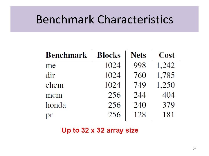
Benchmark Characteristics Up to 32 x 32 array size 23

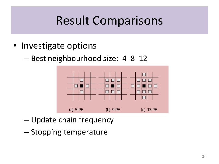
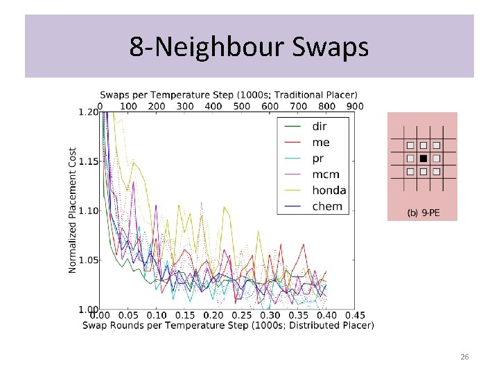
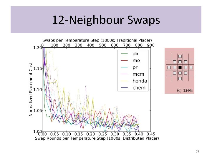
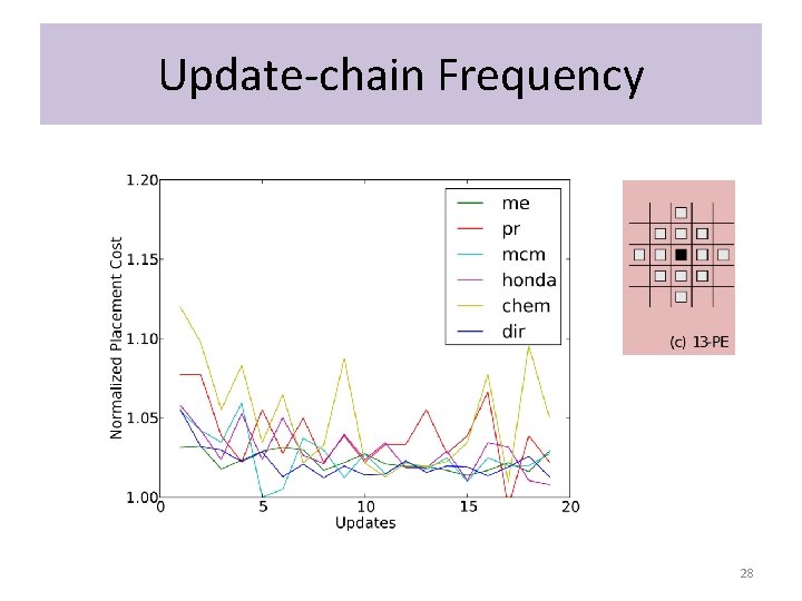
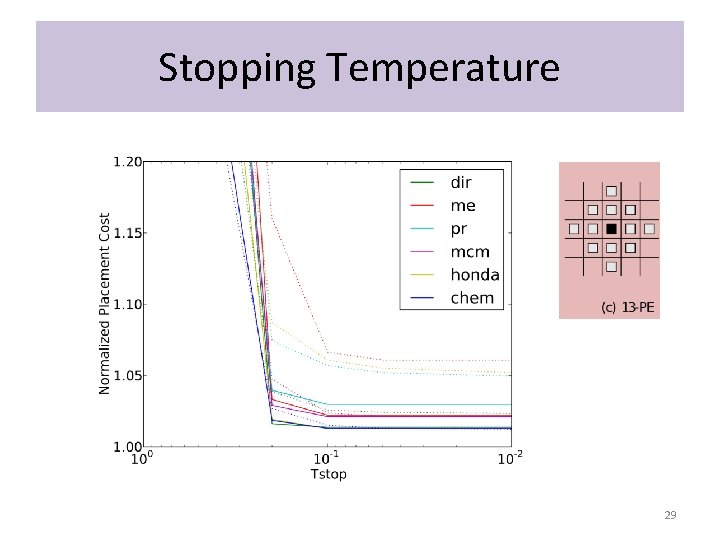
Result Comparisons • Investigate options – Best neighbourhood size: 4 8 12 – Update chain frequency – Stopping temperature 24

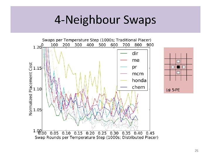
4 -Neighbour Swaps 25

8 -Neighbour Swaps 26

12 -Neighbour Swaps 27

Update-chain Frequency 28

Stopping Temperature 29

Limitations and Future Work • These results were simulated on a PC – Need to target real MPPA – Performance in <# swaps> vs <amount of communication> vs <runtime> • Need to model limited RAM per PE – We assume complete netlist, placement state can be divided among all PEs – Incomplete state if memory is limited? • e. g. , discard some nets? 30

Conclusions • Self-Hosted Simulated Annealing – High-quality placements (within 5%) – Excellent parallelism and speed • Only 1/256 th number of swaps needed – Runs on target architecture itself • Eat you own dog food • Computationally scalable • Memory footprint may not scale to uber-large arrays 31

Conclusions • Self-Hosted Simulated Annealing – High-quality placements (within 5%) – Excellent parallelism and speed • Only 1/256 th number of swaps needed – Runs on target architecture itself • Eat you own dog food • Computationally scalable • Memory footprint may not scale to uber-large arrays • Thank you! 32

EOF 33