Replica Monte Carlo Simulation JianSheng Wang National University

Replica Monte Carlo Simulation Jian-Sheng Wang National University of Singapore 1

Outline • Review of extended ensemble methods (multi-canonical, Wang-Landau, flathistogram, simulated tempering) • Replica MC • Connection to parallel tempering and cluster algorithm of Houdayer • Early and new results 2

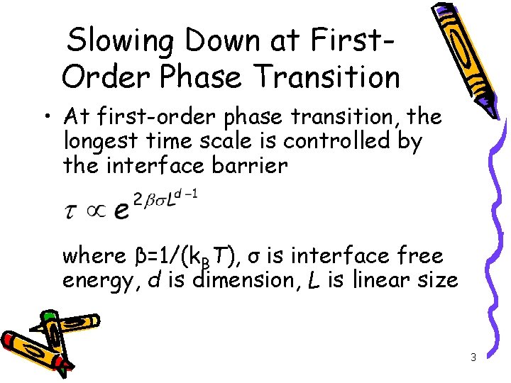
Slowing Down at First. Order Phase Transition • At first-order phase transition, the longest time scale is controlled by the interface barrier where β=1/(k. BT), σ is interface free energy, d is dimension, L is linear size 3

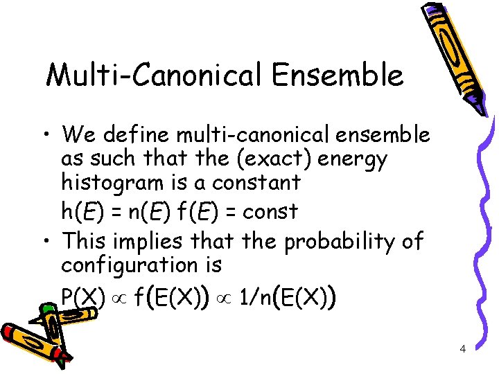
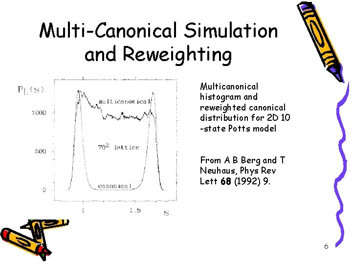
Multi-Canonical Ensemble • We define multi-canonical ensemble as such that the (exact) energy histogram is a constant h(E) = n(E) f(E) = const • This implies that the probability of configuration is P(X) f(E(X)) 1/n(E(X)) 4

Multi-Canonical Simulation (Berg et al) • Do simulation with probability weight fn(E), using Metropolis acceptance rate min[1, fn(E’)/fn(E) ] • Collection histogram H(E) • Re-compute weight by fn+1(E) = fn(E)/H(E) • Iterate until H(E) is flat 5

Multi-Canonical Simulation and Reweighting Multicanonical histogram and reweighted canonical distribution for 2 D 10 -state Potts model From A B Berg and T Neuhaus, Phys Rev Lett 68 (1992) 9. 6

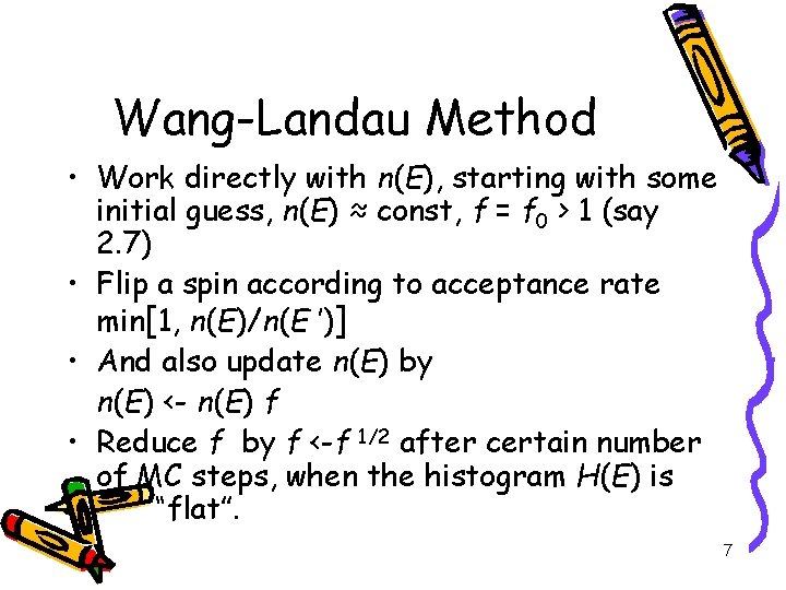
Wang-Landau Method • Work directly with n(E), starting with some initial guess, n(E) ≈ const, f = f 0 > 1 (say 2. 7) • Flip a spin according to acceptance rate min[1, n(E)/n(E ’)] • And also update n(E) by n(E) <- n(E) f • Reduce f by f <-f 1/2 after certain number of MC steps, when the histogram H(E) is “flat”. 7

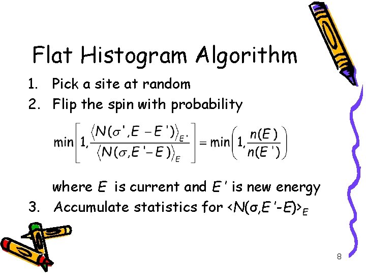
Flat Histogram Algorithm 1. Pick a site at random 2. Flip the spin with probability where E is current and E ’ is new energy 3. Accumulate statistics for <N(σ, E ’-E)>E 8

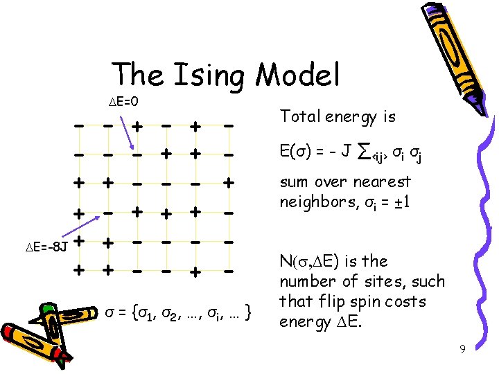
The Ising Model + + DE=-8 J + + DE=0 + + + - σ = {σ1, σ2, …, σi, … } Total energy is E(σ) = - J ∑<ij> σi σj sum over nearest neighbors, σi = ± 1 N(s, DE) is the number of sites, such that flip spin costs energy DE. 9

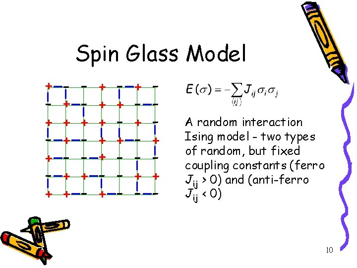
Spin Glass Model + - + + + - + - + + - - + - + - + + - - A random interaction Ising model - two types of random, but fixed coupling constants (ferro Jij > 0) and (anti-ferro Jij < 0) 10

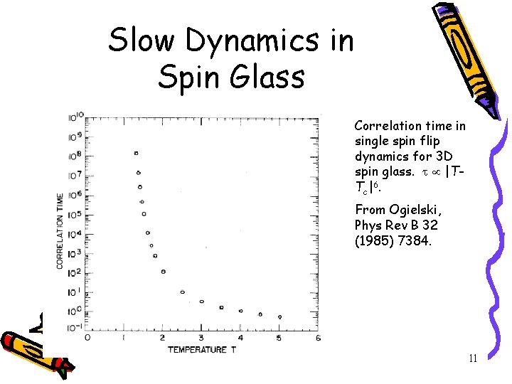
Slow Dynamics in Spin Glass Correlation time in single spin flip dynamics for 3 D spin glass. |TT c | 6. From Ogielski, Phys Rev B 32 (1985) 7384. 11

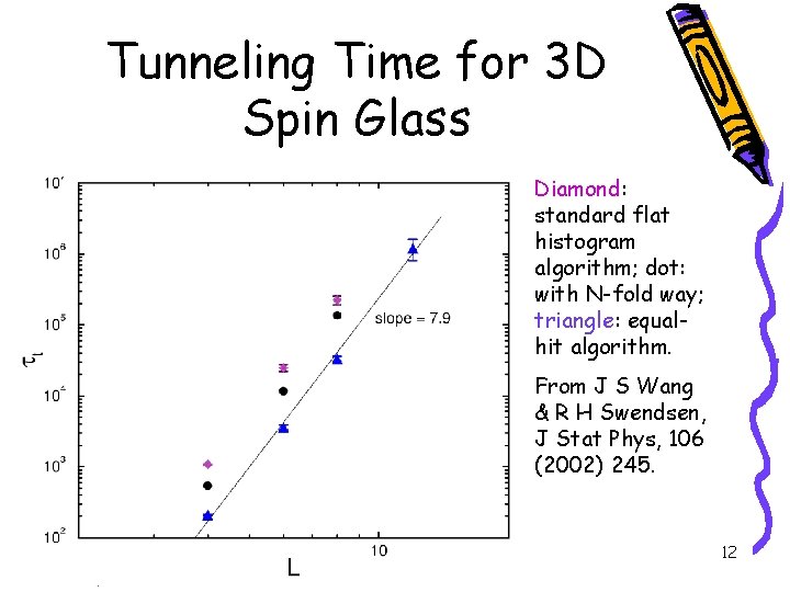
Tunneling Time for 3 D Spin Glass Diamond: standard flat histogram algorithm; dot: with N-fold way; triangle: equalhit algorithm. From J S Wang & R H Swendsen, J Stat Phys, 106 (2002) 245. 12

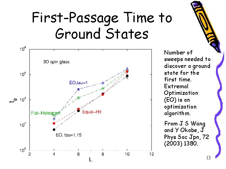
First-Passage Time to Ground States Number of sweeps needed to discover a ground state for the first time. Extremal Optimization (EO) is an optimization algorithm. From J S Wang and Y Okabe, J Phys Soc Jpn, 72 (2003) 1380. 13

Simulated Tempering (Marinari & Parisi, 1992) • Simulated tempering treats parameters as dynamical variables, e. g. , β jumps among a set of values βi. We enlarge sample space as {X, βi}, and make move {X, βi} -> {X’, β’i} according to the usual Metropolis rate. 14

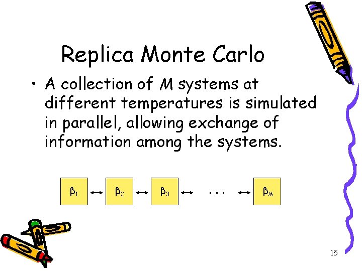
Replica Monte Carlo • A collection of M systems at different temperatures is simulated in parallel, allowing exchange of information among the systems. β 1 β 2 β 3 . . . βM 15

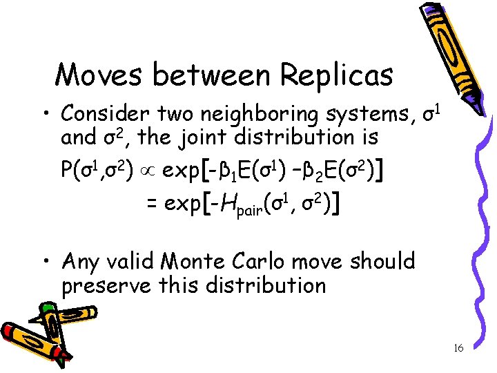
Moves between Replicas • Consider two neighboring systems, σ1 and σ2, the joint distribution is P(σ1, σ2) exp[-β 1 E(σ1) –β 2 E(σ2)] = exp[-Hpair(σ1, σ2)] • Any valid Monte Carlo move should preserve this distribution 16

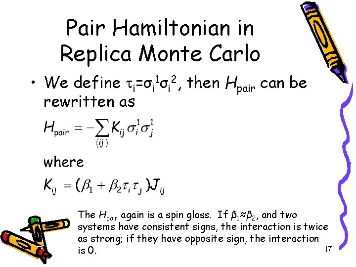
Pair Hamiltonian in Replica Monte Carlo • We define i=σi 1σi 2, then Hpair can be rewritten as The Hpair again is a spin glass. If β 1≈β 2, and two systems have consistent signs, the interaction is twice as strong; if they have opposite sign, the interaction 17 is 0.

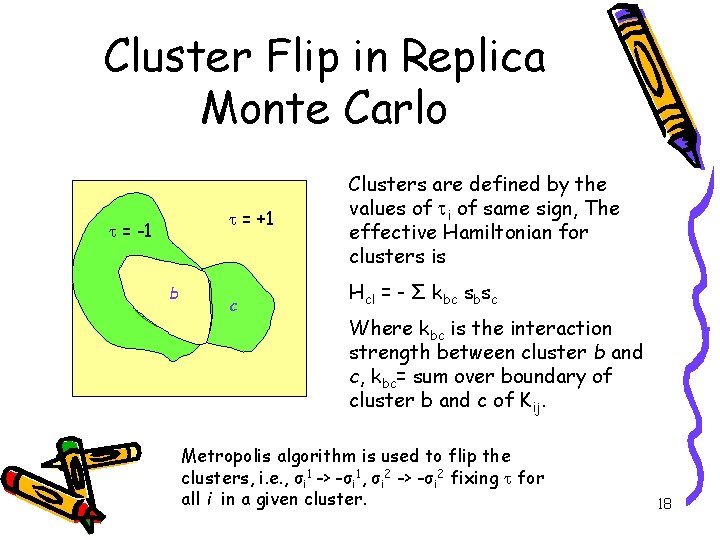
Cluster Flip in Replica Monte Carlo = +1 = -1 b c Clusters are defined by the values of i of same sign, The effective Hamiltonian for clusters is Hcl = - Σ kbc sbsc Where kbc is the interaction strength between cluster b and c, kbc= sum over boundary of cluster b and c of Kij. Metropolis algorithm is used to flip the clusters, i. e. , σi 1 -> -σi 1, σi 2 -> -σi 2 fixing for all i in a given cluster. 18

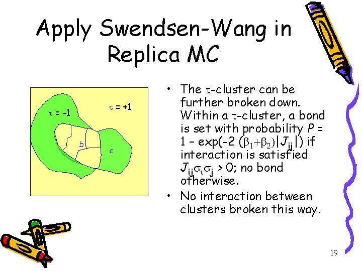
Apply Swendsen-Wang in Replica MC = +1 = -1 b c • The -cluster can be further broken down. Within a -cluster, a bond is set with probability P = 1 – exp(-2 (b 1+b 2)|Jij|) if interaction is satisfied Jijsisj > 0; no bond otherwise. • No interaction between clusters broken this way. 19

Implementation Issues • Use Hoshen-Kompelman algorithm to identify clusters • Based on cluster size and total number of clusters, pre-allocate memory to store effective cluster coupling kab • Order O(N) algorithm for each sweep 20

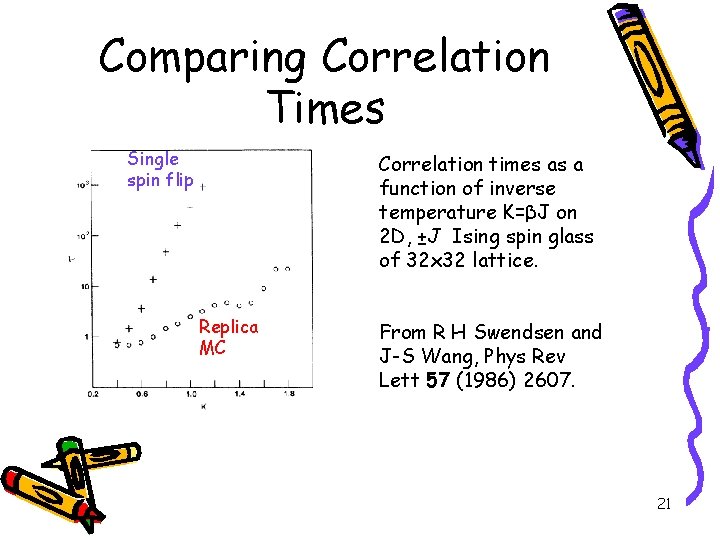
Comparing Correlation Times Single spin flip Correlation times as a function of inverse temperature K=βJ on 2 D, ±J Ising spin glass of 32 x 32 lattice. Replica MC From R H Swendsen and J-S Wang, Phys Rev Lett 57 (1986) 2607. 21

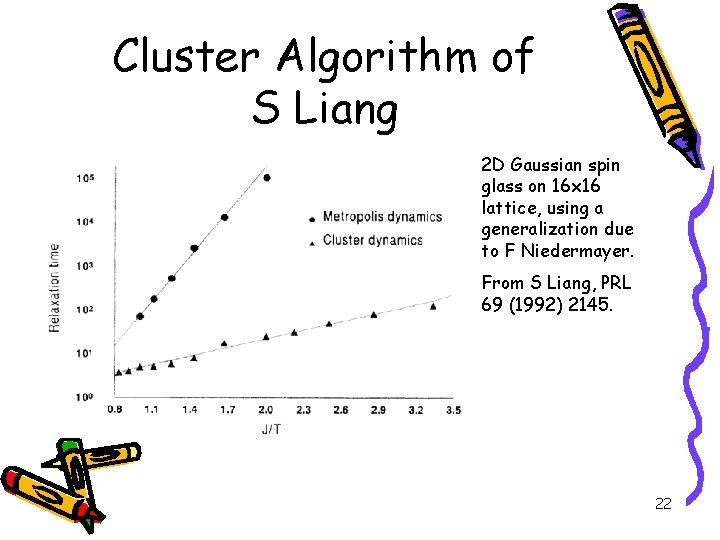
Cluster Algorithm of S Liang 2 D Gaussian spin glass on 16 x 16 lattice, using a generalization due to F Niedermayer. From S Liang, PRL 69 (1992) 2145. 22

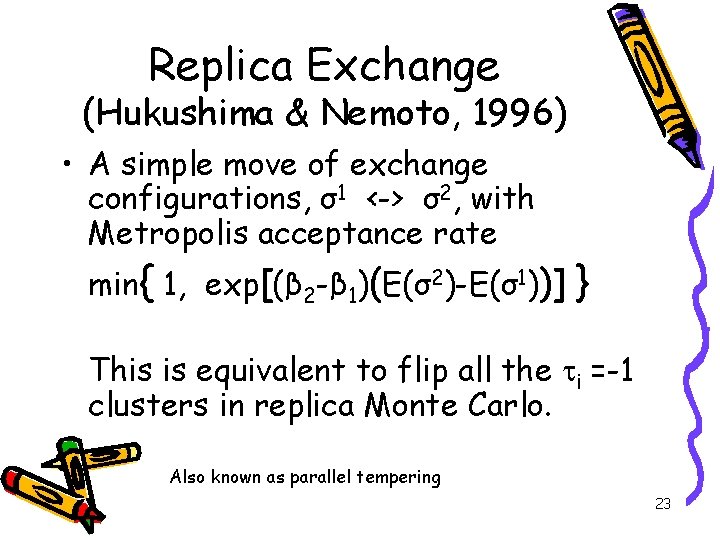
Replica Exchange (Hukushima & Nemoto, 1996) • A simple move of exchange configurations, σ1 <-> σ2, with Metropolis acceptance rate min{ 1, exp[(β 2 -β 1)(E(σ2)-E(σ1))] } This is equivalent to flip all the i =-1 clusters in replica Monte Carlo. Also known as parallel tempering 23

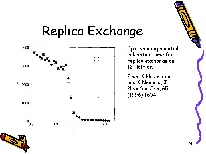
Replica Exchange Spin-spin exponential relaxation time for replica exchange on 123 lattice. From K Hukushima and K Nemoto, J Phys Soc Jpn, 65 (1996) 1604. 24

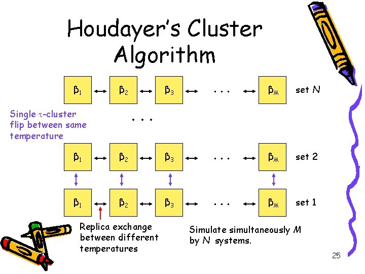
Houdayer’s Cluster Algorithm β 1 β 2 β 3 . . . βM set N . . . Single -cluster flip between same temperature β 1 β 2 β 3 . . . βM set 2 β 1 β 2 β 3 . . . βM set 1 Replica exchange between different temperatures Simulate simultaneously M by N systems. 25

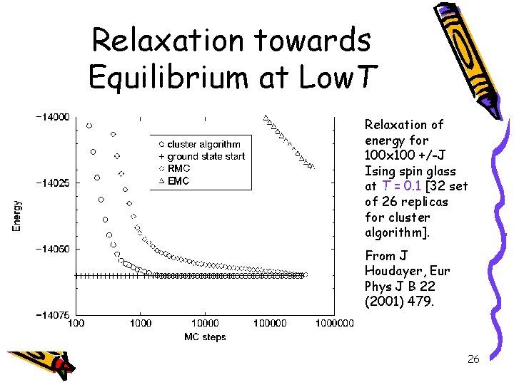
Relaxation towards Equilibrium at Low. T Relaxation of energy for 100 x 100 +/-J Ising spin glass at T = 0. 1 [32 set of 26 replicas for cluster algorithm]. From J Houdayer, Eur Phys J B 22 (2001) 479. 26

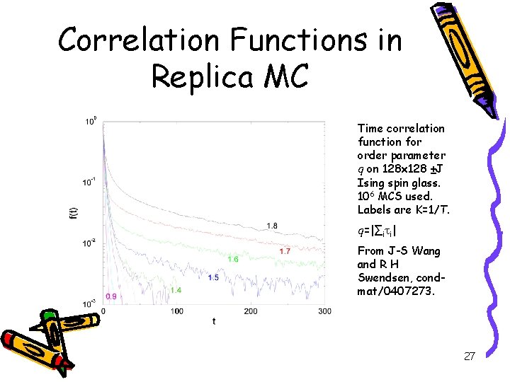
Correlation Functions in Replica MC Time correlation function for order parameter q on 128 x 128 ±J Ising spin glass. 106 MCS used. Labels are K=1/T. q=|∑i i| From J-S Wang and R H Swendsen, condmat/0407273. 27

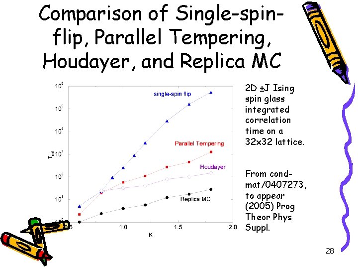
Comparison of Single-spinflip, Parallel Tempering, Houdayer, and Replica MC 2 D ±J Ising spin glass integrated correlation time on a 32 x 32 lattice. From condmat/0407273, to appear (2005) Prog Theor Phys Suppl. 28

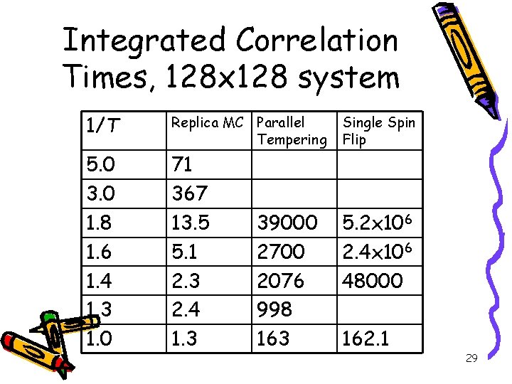
Integrated Correlation Times, 128 x 128 system 1/T Replica MC Parallel Tempering Single Spin Flip 5. 0 3. 0 1. 8 1. 6 1. 4 1. 3 1. 0 71 367 13. 5 5. 1 2. 3 2. 4 1. 3 5. 2 x 106 2. 4 x 106 48000 39000 2700 2076 998 163 162. 1 29

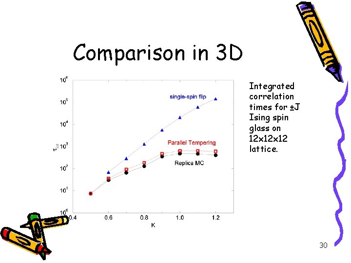
Comparison in 3 D Integrated correlation times for ±J Ising spin glass on 12 x 12 lattice. 30

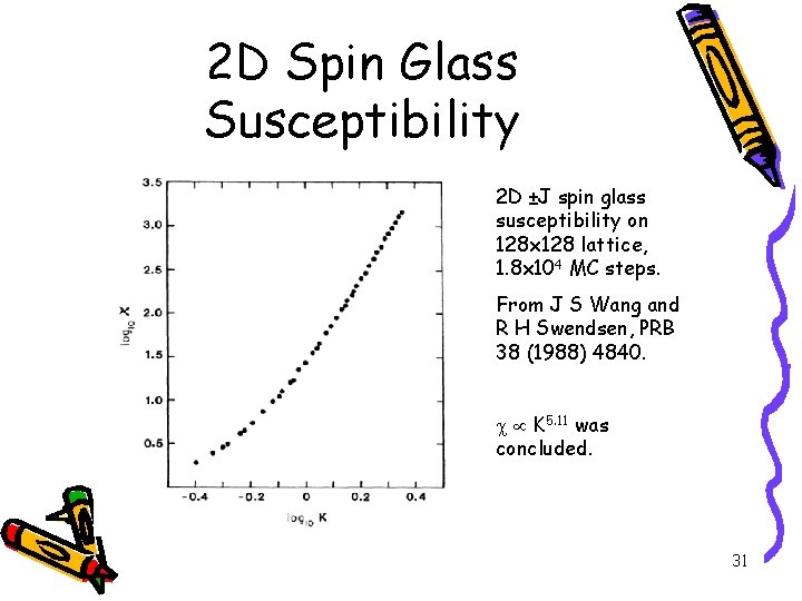
2 D Spin Glass Susceptibility 2 D ±J spin glass susceptibility on 128 x 128 lattice, 1. 8 x 104 MC steps. From J S Wang and R H Swendsen, PRB 38 (1988) 4840. K 5. 11 was concluded. 31

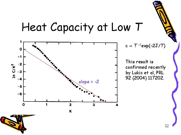
Heat Capacity at Low T c T -2 exp(-2 J/T) slope = -2 This result is confirmed recently by Lukic et al, PRL 92 (2004) 117202. 32

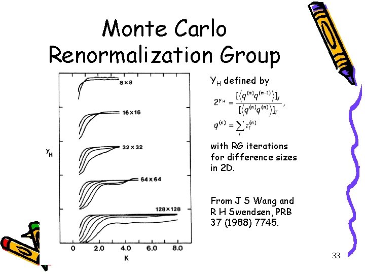
Monte Carlo Renormalization Group YH defined by with RG iterations for difference sizes in 2 D. From J S Wang and R H Swendsen, PRB 37 (1988) 7745. 33

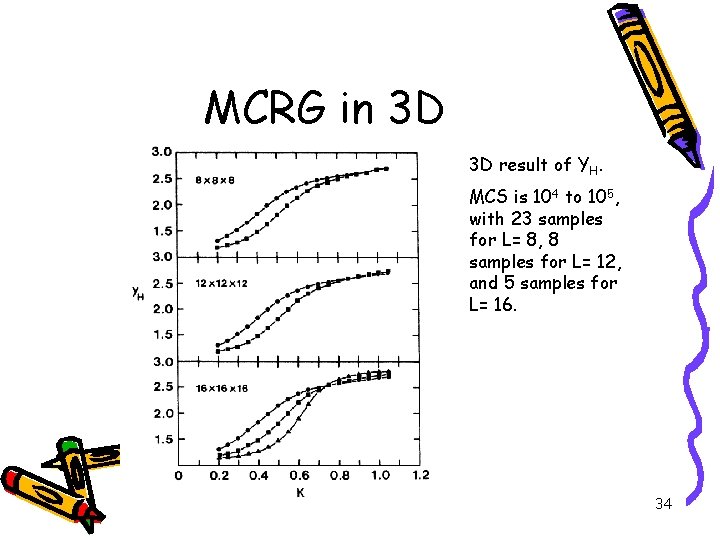
MCRG in 3 D 3 D result of YH. MCS is 104 to 105, with 23 samples for L= 8, 8 samples for L= 12, and 5 samples for L= 16. 34

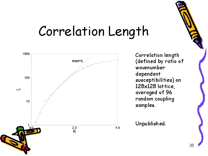
Correlation Length Correlation length (defined by ratio of wavenumber dependent susceptibilities) on 128 x 128 lattice, averaged of 96 random coupling samples. Unpublished. 35

Summary • Replica MC is very efficient in 2 D, and becomes equivalent to Parallel Tempering in 3 D • Replica MC has been used for equilibrium simulations (heat capacity, MCRG, etc) 36