Remote Sensing Image Enhancement Image Enhancement Increases distinction

Remote Sensing Image Enhancement

Image Enhancement ► Increases distinction between features in a scene Single image manipulation ► Multi-image manipulation ►

Single Image ► ► Contrast manipulation Spatial feature manipulation

1. Contrast Manipulation Gray-level threshold ► Level slicing ► Contrast stretching ► Histogram-equalized stretching ►

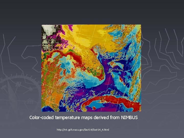
Contrast Manipulation. . Gray-level threshold segmenting an image into two classes - binary mask ► Level slicing dividing the histogram of DNs into several slices ►

Color-coded temperature maps derived from NIMBUS http: //rst. gsfc. nasa. gov/Sect 14_4. html

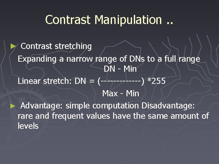
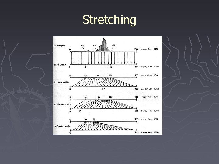
Contrast Manipulation. . ► Contrast stretching Expanding a narrow range of DNs to a full range DN - Min Linear stretch: DN = (-------) *255 Max - Min ► Advantage: simple computation Disadvantage: rare and frequent values have the same amount of levels

Stretching

Contrast Manipulation. . Histogram-equalized stretching ► Stretch based on frequency of occurrence ► Frequently occurred DNs have more display levels ► ► Special stretch

2. Spatial Feature Manipulation Spatial filtering ► Edge enhancement ► Convolution ► Directional first differencing ►

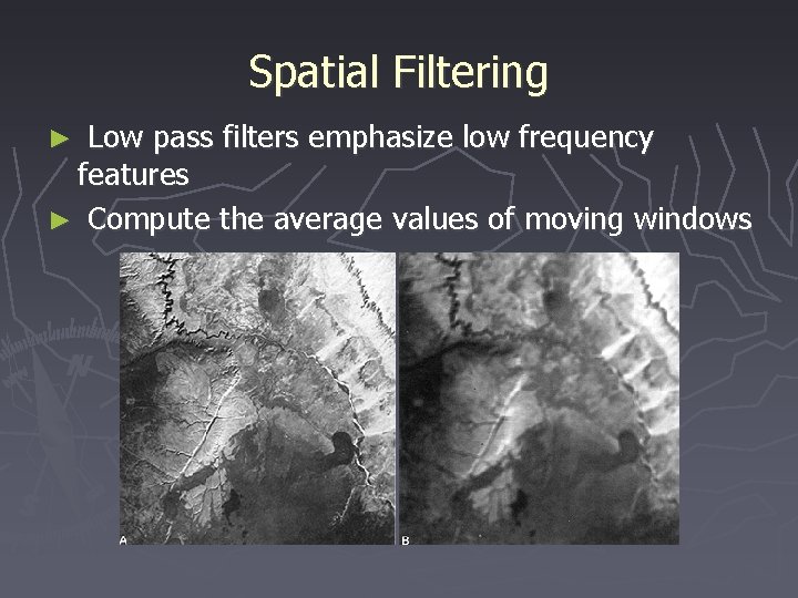
Spatial Filtering Low pass filters emphasize low frequency features ► Compute the average values of moving windows ►

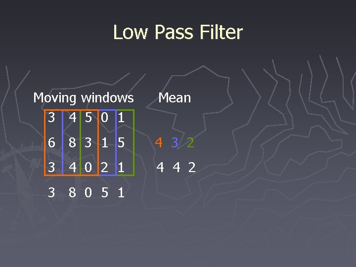
Low Pass Filter Moving windows 3 4 5 0 1 Mean 6 8 3 1 5 4 3 2 3 4 0 2 1 4 4 2 3 8 0 5 1

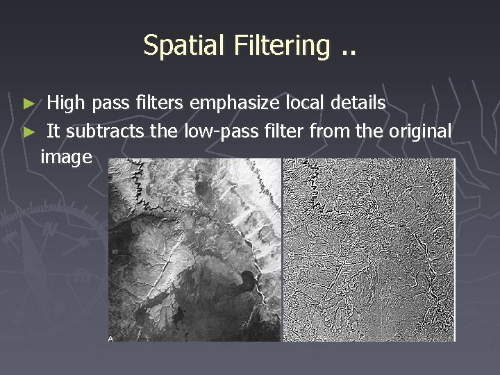
Spatial Filtering. . High pass filters emphasize local details ► It subtracts the low-pass filter from the original image ►

Edge Enhancement Add back the high frequency image component to the original image ► Preserve both the original and the high frequency features ►

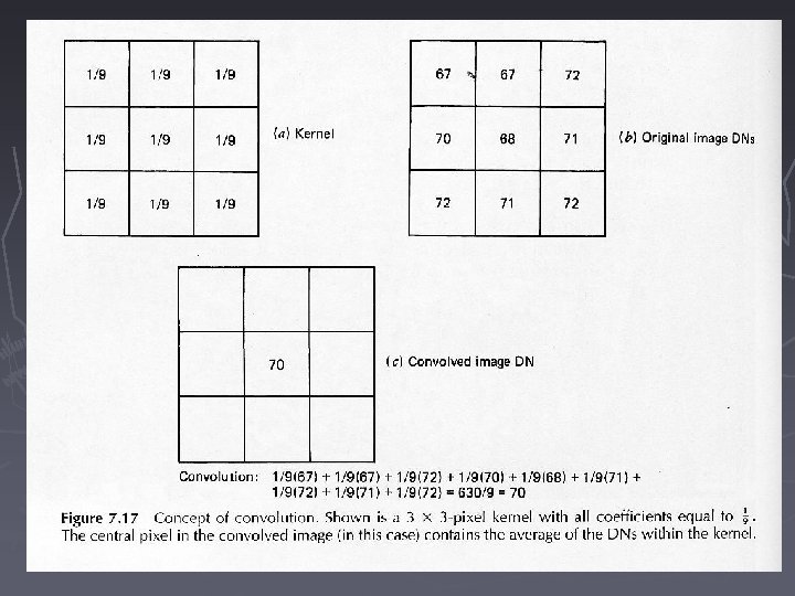
Convolution ► A moving kernel with a weighting factor for each pixel

Convolution

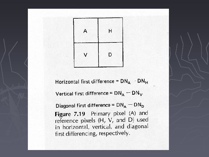
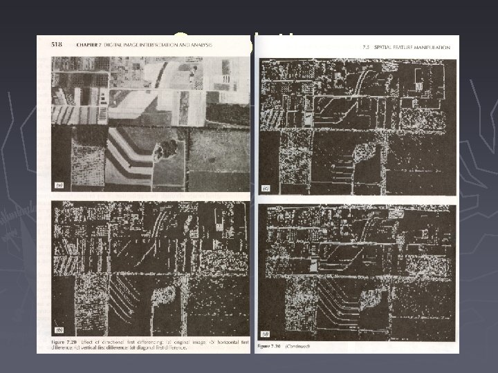
Directional Differencing Displaying the differences in gray levels of adjacent pixels ► The direction can be horizontal, vertical, or diagonal ► It is necessary to add a constant to the difference for display purposes ► Add back the directional difference to the original image ► ► Contrast stretching is needed for all feature manipulations

Convolution

3. Multi-image Manipulation ► ► Spectral ratioing Principle component transformation Kauth-Thomas tasseled cap Intensity-Hue-Saturation transformation (IHS)

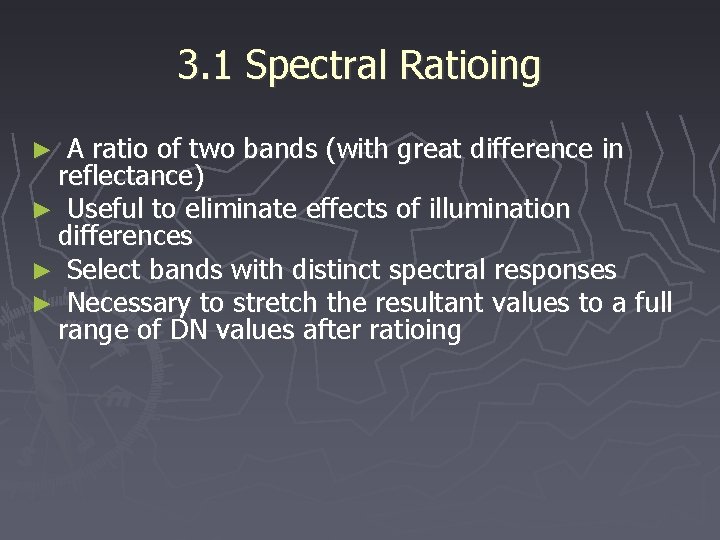
3. 1 Spectral Ratioing A ratio of two bands (with great difference in reflectance) ► Useful to eliminate effects of illumination differences ► Select bands with distinct spectral responses ► Necessary to stretch the resultant values to a full range of DN values after ratioing ►

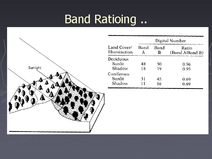
Band Ratioing. .

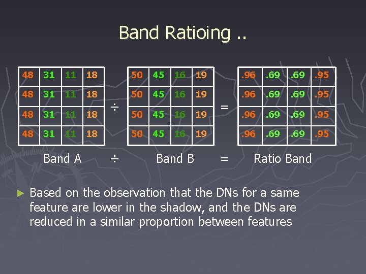
Band Ratioing. . 48 31 11 18 50 45 16 19 . 96 . 69 . 95 Band A ► ÷ ÷ Band B = = Ratio Band Based on the observation that the DNs for a same feature are lower in the shadow, and the DNs are reduced in a similar proportion between features

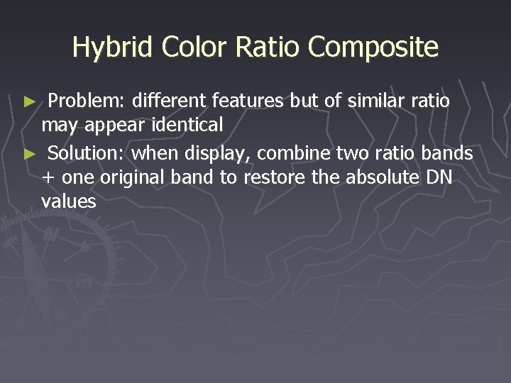
Hybrid Color Ratio Composite Problem: different features but of similar ratio may appear identical ► Solution: when display, combine two ratio bands + one original band to restore the absolute DN values ►

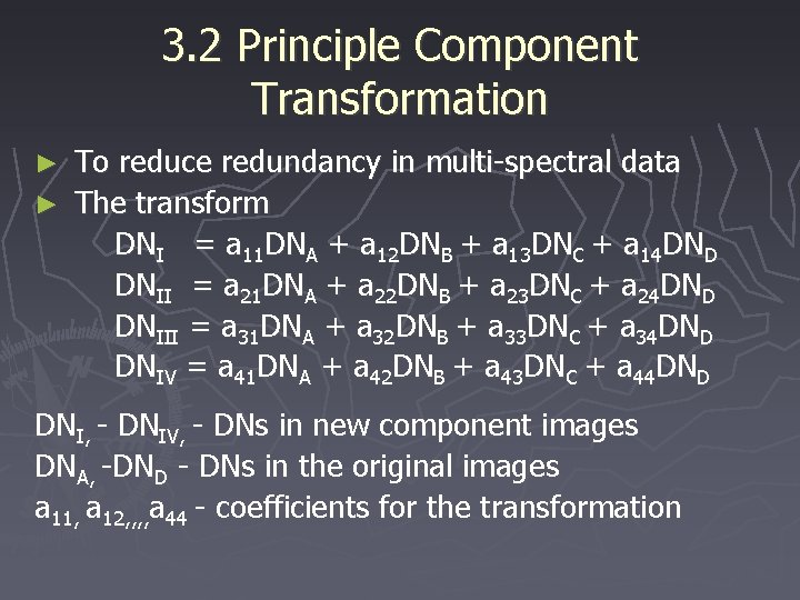
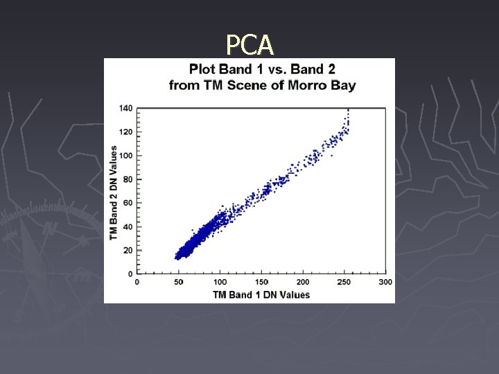
3. 2 Principle Component Transformation To reduce redundancy in multi-spectral data ► The transform DNI = a 11 DNA + a 12 DNB + a 13 DNC + a 14 DND DNII = a 21 DNA + a 22 DNB + a 23 DNC + a 24 DND DNIII = a 31 DNA + a 32 DNB + a 33 DNC + a 34 DND DNIV = a 41 DNA + a 42 DNB + a 43 DNC + a 44 DND ► DNI, - DNIV, - DNs in new component images DNA, -DND - DNs in the original images a 11, a 12, , a 44 - coefficients for the transformation

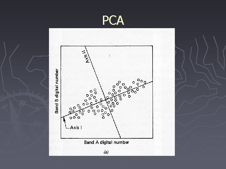
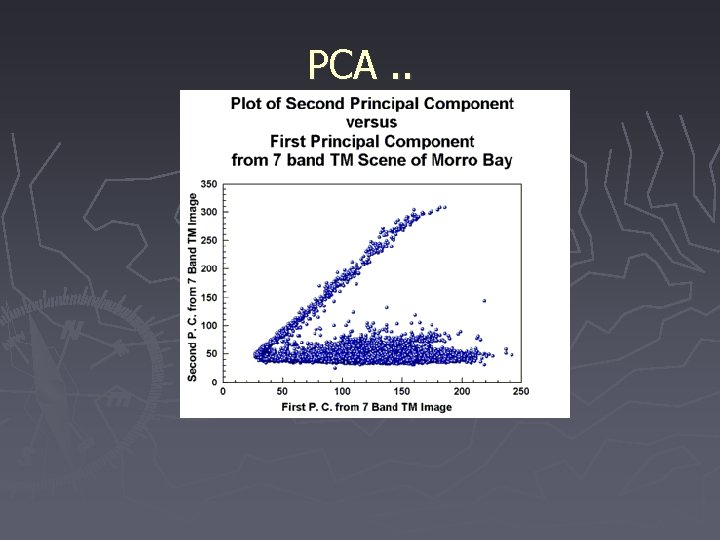
PCA

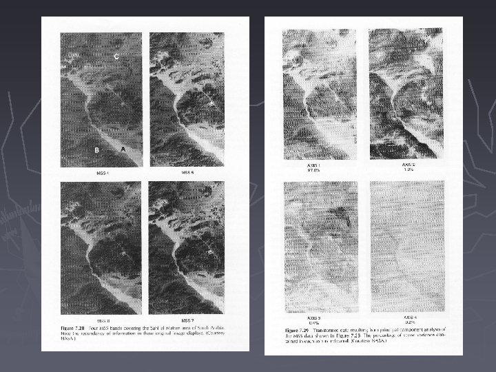
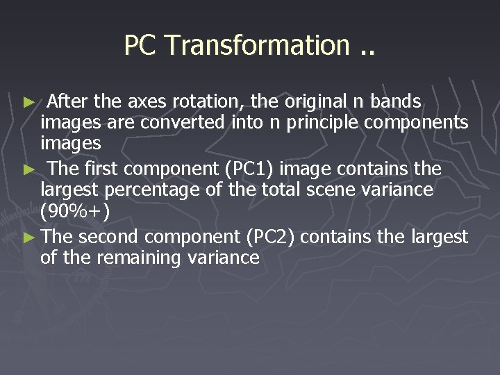
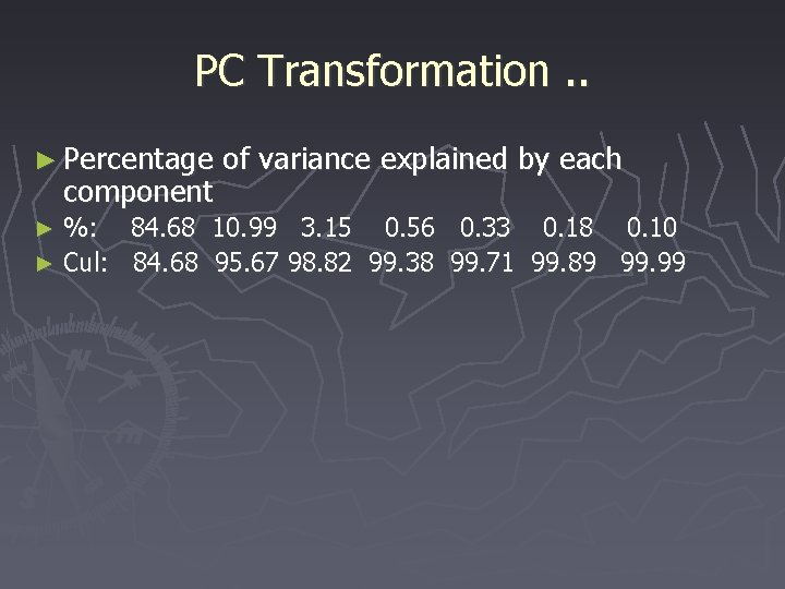
PC Transformation. . After the axes rotation, the original n bands images are converted into n principle components images ► The first component (PC 1) image contains the largest percentage of the total scene variance (90%+) ► The second component (PC 2) contains the largest of the remaining variance ►

PC Transformation. . ► Percentage component of variance explained by each %: 84. 68 10. 99 3. 15 0. 56 0. 33 0. 18 0. 10 ► Cul: 84. 68 95. 67 98. 82 99. 38 99. 71 99. 89 99. 99 ►

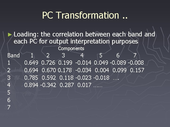
PC Transformation. . ► Loading: the correlation between each band each PC for output interpretation purposes Components Band 1 2 3 4 5 6 7 0. 649 0. 726 0. 199 -0. 014 0. 049 -0. 089 -0. 008 0. 694 0. 670 0. 178 -0. 034 0. 004 0. 099 0. 157 0. 785 0. 592 0. 118 -0. 023 -0. 018 …. 0. 894 -0. 342 0. 287 0. 017 ……

PCA

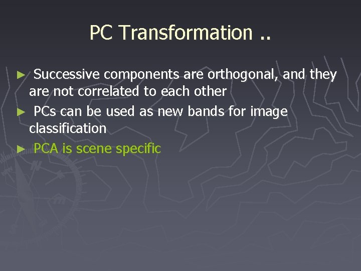
PC Transformation. . Successive components are orthogonal, and they are not correlated to each other ► PCs can be used as new bands for image classification ► PCA is scene specific ►

3. 3 Kauth-Thomas Tasseled Cap An orthogonal transformation ► The 4 MSS bands can be converted into 4 new bands: brightness greenness yellow stuff non-such ►

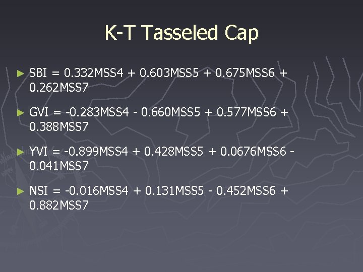
K-T Tasseled Cap ► SBI = 0. 332 MSS 4 + 0. 603 MSS 5 + 0. 675 MSS 6 + 0. 262 MSS 7 ► GVI = -0. 283 MSS 4 - 0. 660 MSS 5 + 0. 577 MSS 6 + 0. 388 MSS 7 ► YVI = -0. 899 MSS 4 + 0. 428 MSS 5 + 0. 0676 MSS 6 0. 041 MSS 7 ► NSI = -0. 016 MSS 4 + 0. 131 MSS 5 - 0. 452 MSS 6 + 0. 882 MSS 7

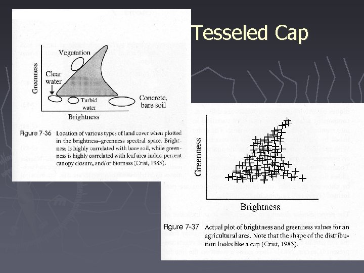
Kauth-Thomas Tasseled Cap The first two indices contain the most info (90%+) ► Brightness is related to bare soils ► Greenness is related to the amount of green vegetation ►

Kauth-Thomas Tesseled Cap

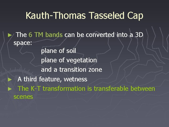
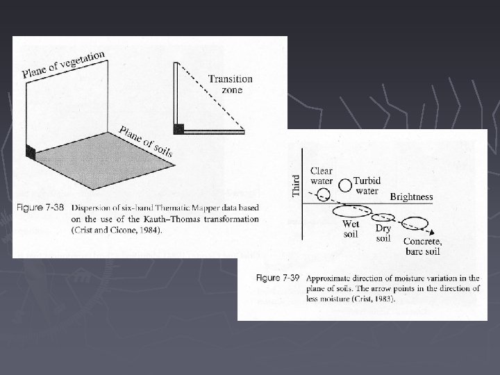
Kauth-Thomas Tasseled Cap The 6 TM bands can be converted into a 3 D space: plane of soil plane of vegetation and a transition zone ► A third feature, wetness ► The K-T transformation is transferable between scenes ►

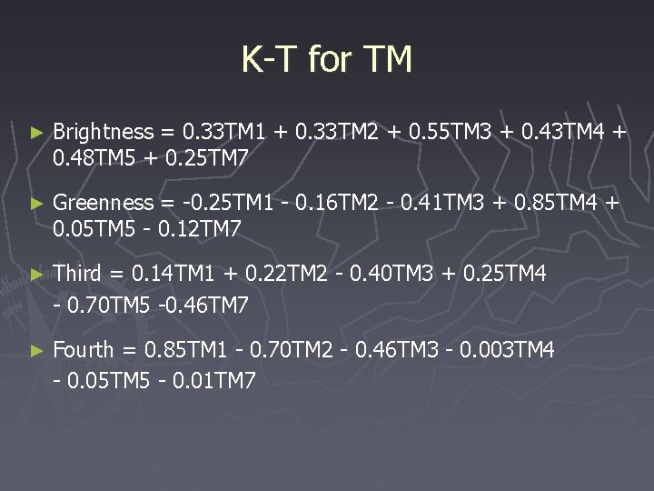
K-T for TM ► Brightness = 0. 33 TM 1 + 0. 33 TM 2 + 0. 55 TM 3 + 0. 43 TM 4 + 0. 48 TM 5 + 0. 25 TM 7 ► Greenness = -0. 25 TM 1 - 0. 16 TM 2 - 0. 41 TM 3 + 0. 85 TM 4 + 0. 05 TM 5 - 0. 12 TM 7 ► Third = 0. 14 TM 1 + 0. 22 TM 2 - 0. 40 TM 3 + 0. 25 TM 4 - 0. 70 TM 5 -0. 46 TM 7 ► Fourth = 0. 85 TM 1 - 0. 70 TM 2 - 0. 46 TM 3 - 0. 003 TM 4 - 0. 05 TM 5 - 0. 01 TM 7

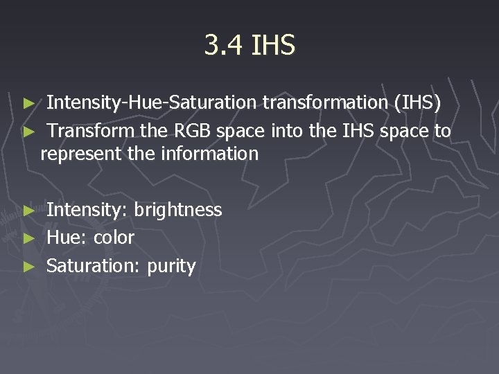
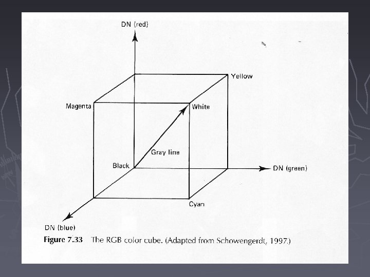
3. 4 IHS Intensity-Hue-Saturation transformation (IHS) ► Transform the RGB space into the IHS space to represent the information ► Intensity: brightness ► Hue: color ► Saturation: purity ►

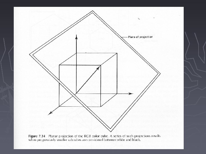
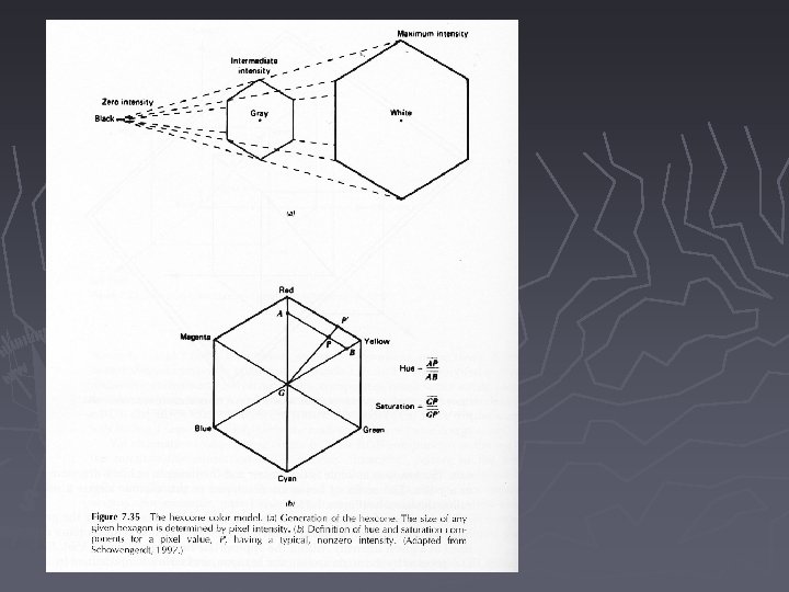
IHS The hexcone model projects the RGB cube to a plane, resulting in a hexagon ► The plane is perpendicular to the gray line and tangent to the cube at the "white" corner ►

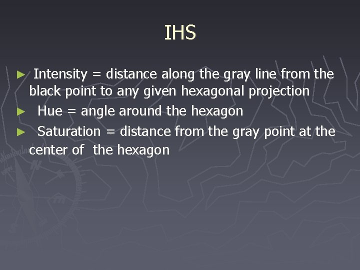
IHS Intensity = distance along the gray line from the black point to any given hexagonal projection ► Hue = angle around the hexagon ► Saturation = distance from the gray point at the center of the hexagon ►

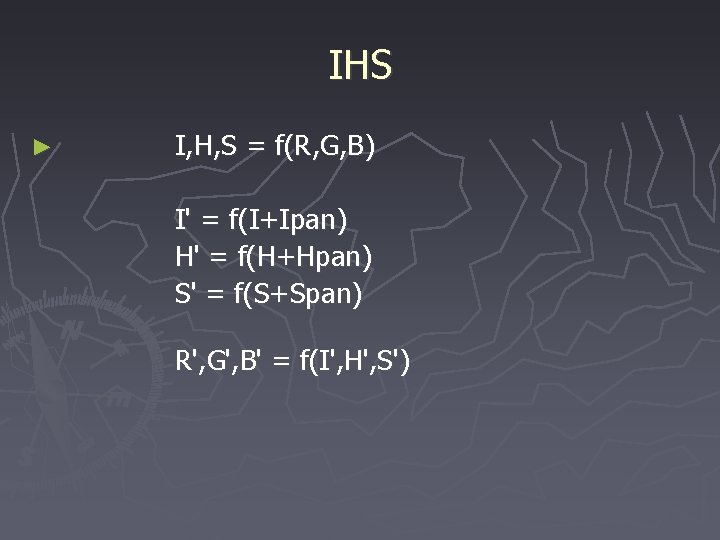
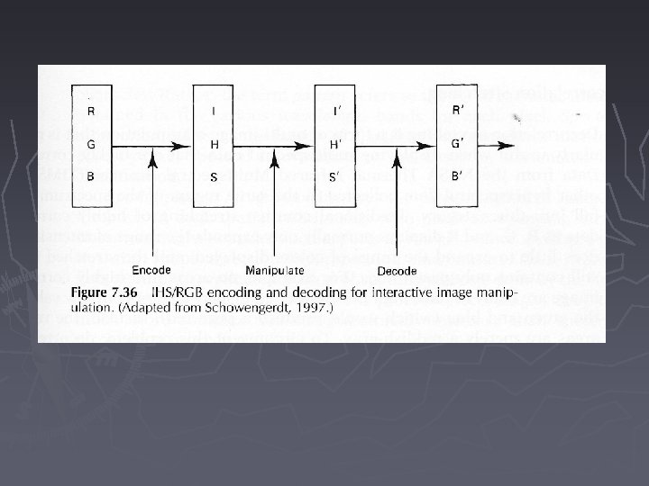
IHS ► I, H, S = f(R, G, B) I' = f(I+Ipan) H' = f(H+Hpan) S' = f(S+Span) R', G', B' = f(I', H', S')

Readings ► Chapter 7

PCA. .