Quick Sort 11 2 CSE 2011 Winter 2011

Quick Sort (11. 2) CSE 2011 Winter 2011 2/22/2021 1

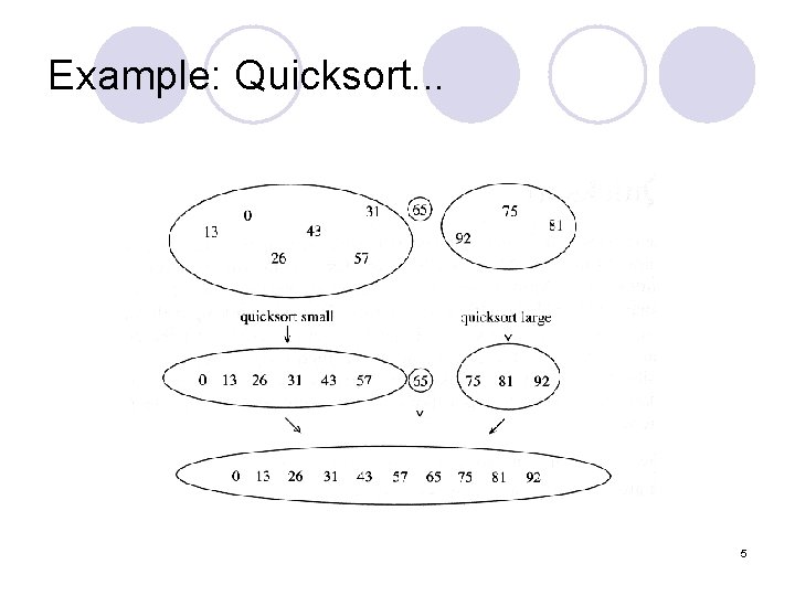
Quick Sort l Fastest known sorting algorithm in practice l Average case: O(N log N) l Worst case: O(N 2) ¡But the worst case can be made exponentially unlikely. l Another divide-and-conquer recursive algorithm, like merge sort 2

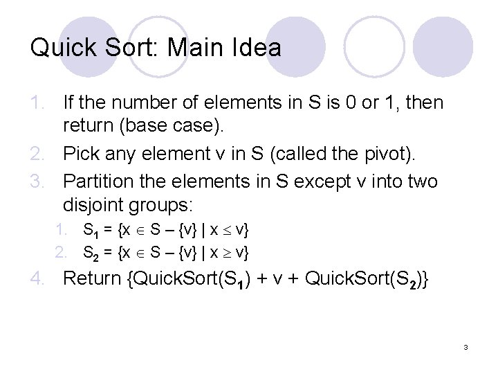
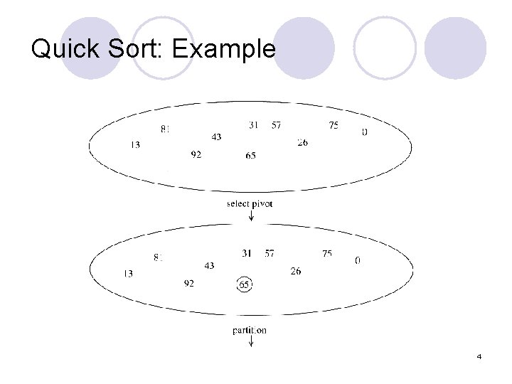
Quick Sort: Main Idea 1. If the number of elements in S is 0 or 1, then return (base case). 2. Pick any element v in S (called the pivot). 3. Partition the elements in S except v into two disjoint groups: 1. S 1 = {x S – {v} | x v} 2. S 2 = {x S – {v} | x v} 4. Return {Quick. Sort(S 1) + v + Quick. Sort(S 2)} 3

Quick Sort: Example 4

Example: Quicksort. . . 5

Issues To Consider l How to pick the pivot? l How to partition? ¡ Several methods exist. ¡ The one we consider is known to give good results and to be easy and efficient. 6

Partitioning Strategy l Want to partition an array A[left. . right] l First, get the pivot element out of the way by swapping it with the last element (swap pivot and A[right]) l Let i start at the first element and j start at the next-tolast element (i = left, j = right – 1) swap 5 7 4 6 pivot 3 12 19 5 i 7 4 19 3 12 6 j 7

Partitioning Strategy l Want to have pivot ¡ A[k] pivot, for k < i ¡ A[k] pivot, for k > j l When i < j j i ¡ Move i right, skipping over elements smaller than the pivot ¡ Move j left, skipping over elements greater than the pivot ¡ When both i and j have stopped l A[i] pivot l A[j] pivot A[i] and A[j] should now be swapped 5 i 7 4 19 3 12 j 6 5 7 i 4 19 3 12 j 6 8

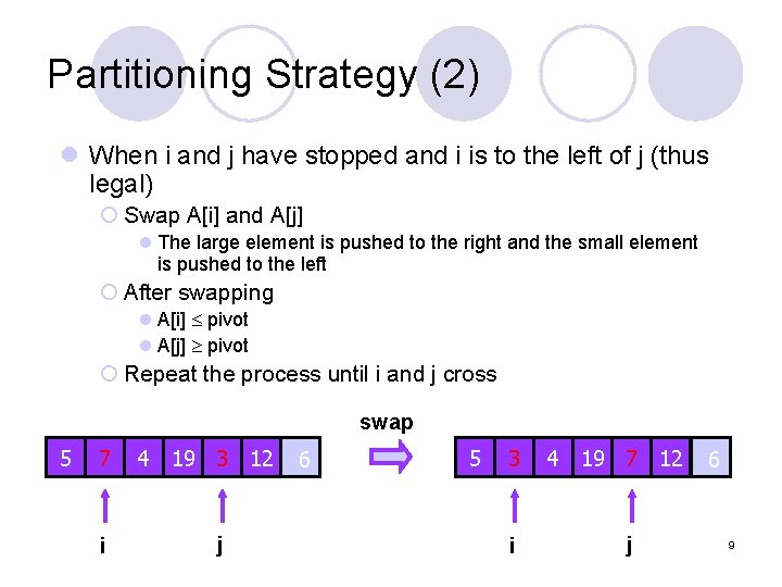
Partitioning Strategy (2) l When i and j have stopped and i is to the left of j (thus legal) ¡ Swap A[i] and A[j] l The large element is pushed to the right and the small element is pushed to the left ¡ After swapping l A[i] pivot l A[j] pivot ¡ Repeat the process until i and j cross swap 5 7 i 4 19 3 12 j 6 5 3 i 4 19 7 12 j 6 9

Partitioning Strategy (3) l When i and j have crossed 5 ¡swap A[i] and pivot l Result: ¡A[k] pivot, for k < i ¡A[k] pivot, for k > i 3 4 19 7 12 j i 5 3 4 19 7 12 Swap! 5 3 Break! 6 i 4 6 j i 6 j 7 12 19 10

Picking the Pivot l Objective: Choose a pivot so that we will get 2 partitions of (almost) equal size.

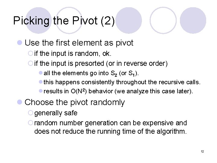
Picking the Pivot (2) l Use the first element as pivot ¡ if the input is random, ok. ¡ if the input is presorted (or in reverse order) l all the elements go into S 2 (or S 1). l this happens consistently throughout the recursive calls. l results in O(N 2) behavior (we analyze this case later). l Choose the pivot randomly ¡ generally safe ¡ random number generation can be expensive and does not reduce the running time of the algorithm. 12

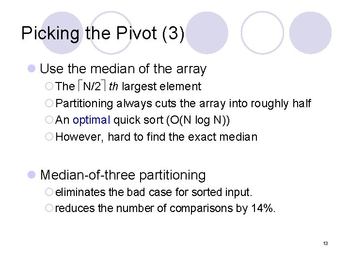
Picking the Pivot (3) l Use the median of the array ¡The N/2 th largest element ¡Partitioning always cuts the array into roughly half ¡An optimal quick sort (O(N log N)) ¡However, hard to find the exact median l Median-of-three partitioning ¡ eliminates the bad case for sorted input. ¡ reduces the number of comparisons by 14%. 13

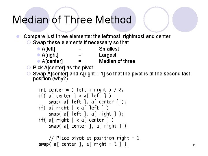
Median of Three Method l Compare just three elements: the leftmost, rightmost and center ¡ Swap these elements if necessary so that l A[left] = Smallest l A[right] = Largest l A[center] = Median of three ¡ Pick A[center] as the pivot. ¡ Swap A[center] and A[right – 1] so that the pivot is at the second last position (why? ) 14

Median of Three: Example A[left] = 2, A[center] = 13, A[right] = 6 2 5 6 4 13 3 12 19 2 5 6 4 6 3 12 19 13 Swap A[center] and A[right] 2 5 6 4 6 3 12 19 13 Choose A[center] as pivot 6 pivot 2 5 6 4 19 3 12 6 13 Swap pivot and A[right – 1] pivot We only need to partition A[ left + 1, …, right – 2 ]. Why? 15

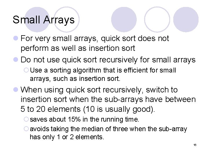
Small Arrays l For very small arrays, quick sort does not perform as well as insertion sort l Do not use quick sort recursively for small arrays ¡Use a sorting algorithm that is efficient for small arrays, such as insertion sort. l When using quick sort recursively, switch to insertion sort when the sub-arrays have between 5 to 20 elements (10 is usually good). ¡ saves about 15% in the running time. ¡ avoids taking the median of three when the sub-array has only 1 or 2 elements. 16

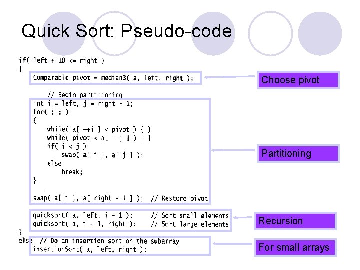
Quick Sort: Pseudo-code Choose pivot Partitioning Recursion For small arrays 17

Partitioning Part l Works only if pivot is picked as median-of-three. ¡ A[left] pivot and A[right] pivot ¡ Need to partition only A[left + 1, …, right – 2] l j will not run past the beginning ¡ because A[left] pivot l i will not run past the end ¡ because A[right-1] = pivot 18

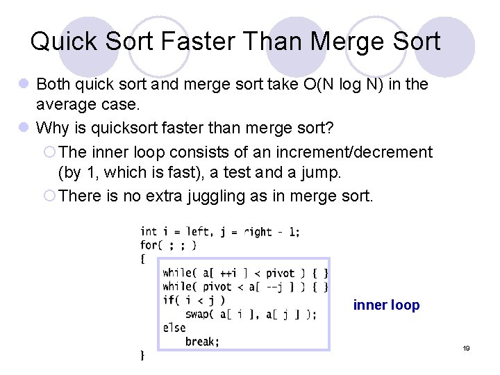
Quick Sort Faster Than Merge Sort l Both quick sort and merge sort take O(N log N) in the average case. l Why is quicksort faster than merge sort? ¡The inner loop consists of an increment/decrement (by 1, which is fast), a test and a jump. ¡There is no extra juggling as in merge sort. inner loop 19

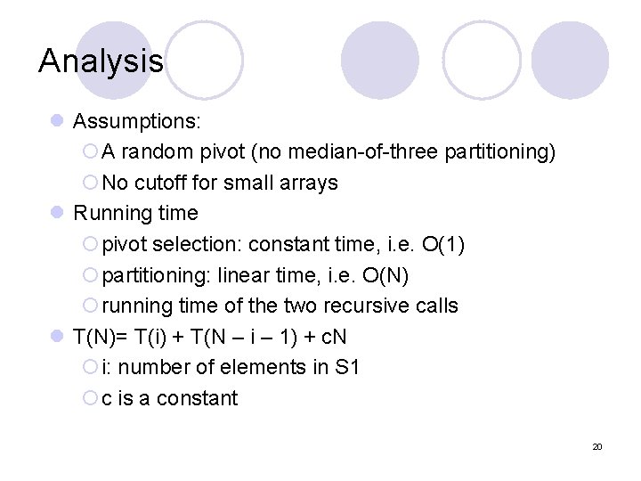
Analysis l Assumptions: ¡A random pivot (no median-of-three partitioning) ¡No cutoff for small arrays l Running time ¡pivot selection: constant time, i. e. O(1) ¡partitioning: linear time, i. e. O(N) ¡running time of the two recursive calls l T(N)= T(i) + T(N – i – 1) + c. N ¡i: number of elements in S 1 ¡c is a constant 20

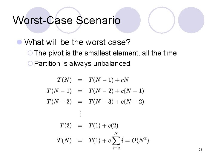
Worst-Case Scenario l What will be the worst case? ¡The pivot is the smallest element, all the time ¡Partition is always unbalanced 21

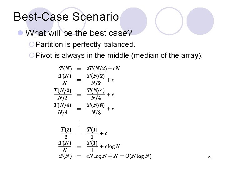
Best-Case Scenario l What will be the best case? ¡Partition is perfectly balanced. ¡Pivot is always in the middle (median of the array). 22

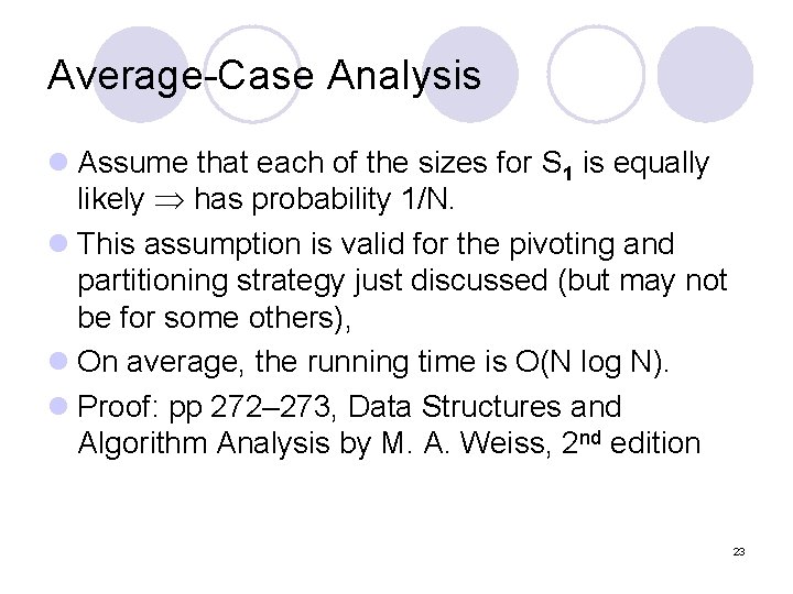
Average-Case Analysis l Assume that each of the sizes for S 1 is equally likely has probability 1/N. l This assumption is valid for the pivoting and partitioning strategy just discussed (but may not be for some others), l On average, the running time is O(N log N). l Proof: pp 272– 273, Data Structures and Algorithm Analysis by M. A. Weiss, 2 nd edition 23

Next time … l Arrays (review) l Linked Lists (3. 2, 3. 3) l Stacks, queues (Chapter 5) 24