Sorting n Popular algorithms Selection sort Insertion sort

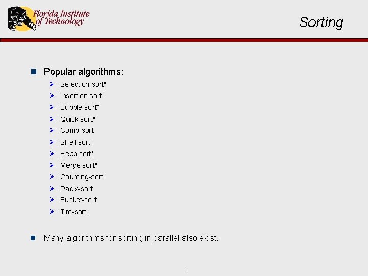
Sorting n Popular algorithms: Ø Ø Ø Selection sort* Insertion sort* Bubble sort* Quick sort* Comb-sort Shell-sort Heap sort* Merge sort* Counting-sort Radix-sort Bucket-sort Tim-sort n Many algorithms for sorting in parallel also exist. 1

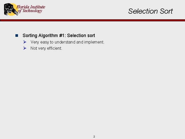
Selection Sorting Algorithm #1: Selection sort Ø Very easy to understand implement. Ø Not very efficient. 2

Selection Sort // Selection sort in Java public static void sort(int[] a){ int min. Pos, temp; for (int i=0; i<=a. length-2; i++){ // Find the position of the value that belongs in position i min. Pos = i; for (int j=i+1; j<=a. length-1; j++) if (a[j] < a[min. Pos]) min. Pos = j; // Swap the values in positions i and min temp = a[i]; a[i] = a[min. Pos]; a[min. Pos] = temp; Running time? } } Θ(n 2) – best, worst, average 3

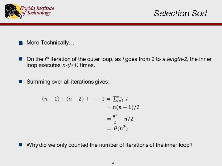
Selection Sort n 4

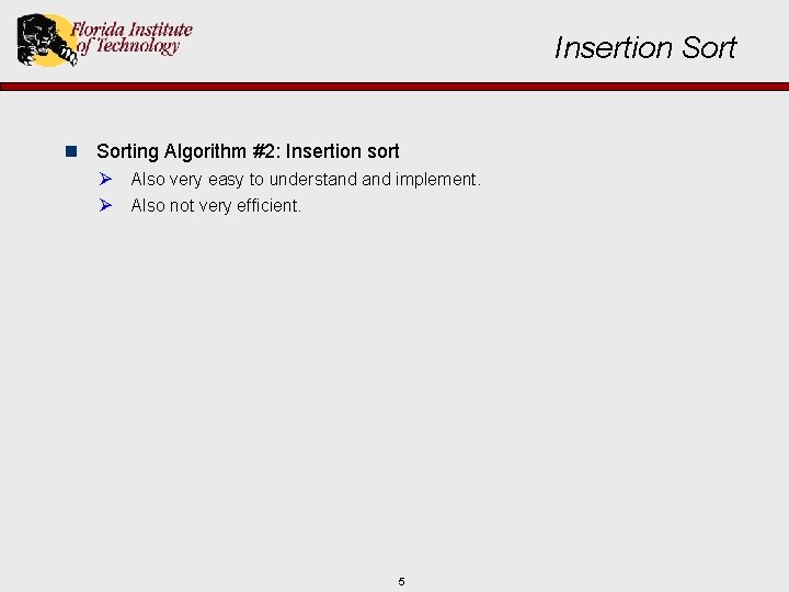
Insertion Sorting Algorithm #2: Insertion sort Ø Also very easy to understand implement. Ø Also not very efficient. 5

Insertion Sort n Initial version: // Insertion sort public static void insertion. Sort(int[] a) { int j; for (int i=1; i<=a. length-1; i++) { j=i; while (j>=1) { if (a[j] < a[j-1]) { temp=a[j-1]; a[j-1]=a[j]; a[j]=temp; } j=j-1; } Running time? Θ(n 2) – best, worst, average Analysis is same as for Selection-sort } } 6

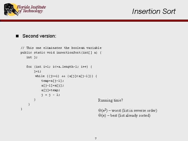
Insertion Sort n Second version: // This one eliminates the boolean variable public static void insertion. Sort(int[] a) { int j; for (int i=1; i<=a. length-1; i++) { j=i; while ((j>=1) && (a[j]<a[j-1])) { temp=a[j-1]; a[j-1]=a[j]; a[j]=temp; j = j – 1; } } } Running time? Θ(n 2) – worst (list in reverse order) Θ(n) – best (list already sorted) 7

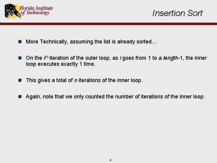
Insertion Sort n More Technically, assuming the list is already sorted… n On the ith iteration of the outer loop, as i goes from 1 to a. length-1, the inner loop executes exactly 1 time. n This gives a total of n iterations of the inner loop. n Again, note that we only counted the number of iterations of the inner loop. 8

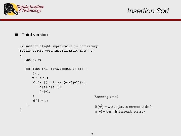
Insertion Sort n Third version: // Another slight improvement in efficiency public static void insertion. Sort(int[] a) { int j, v; for (int i=1; i<=a. length-1; i++) { j=i; v = a[j]; while ((j>=1) && (v<a[j-1])) { a[j]=a[j-1]; j=j-1; } a[j] = v; } Running time? Θ(n 2) – worst (list in reverse order) Θ(n) – best (list already sorted) } 9

Bubble Sort n Sorting Algorithm #3: Bubble sort Ø Also very easy to understand implement. Ø Also not very efficient. Ø Several minor variations and enhancements are possible. 10

Bubble Sort n Initial version: // Bubble sort public static void bubble. Sort 1(int[] a) { int temp; for (int i=1; i<=a. length-1; i++) { for (int j=0; j<a. length-i; j++) { if (a[j] > a[j+1]) { temp = a[j]; a[j] = a[j+1]; Running time? a[j+1] = temp; } 2 Θ(n ) – best, worst, average Analysis is same as for Selection-sort } } } 11

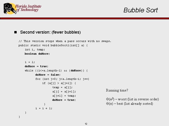
Bubble Sort n Second version: (fewer bubbles) // This version stops when a pass occurs with no swaps. public static void bubble. Sort 1(int[] a) { int i, temp; boolean do. More; i = 1; do. More = true; while ((i<=a. length-1) && ( do. More)) { do. More = false; for (int j=0; j<a. length-i; j++) if (a[j] > a[j+1]) { temp = a[j]; a[j] = a[j+1]; a[j+1] = temp; do. More = true; } i = i + 1; } } 12 Running time? Θ(n 2) – worst (list in reverse order) Θ(n) – best (list already sorted)

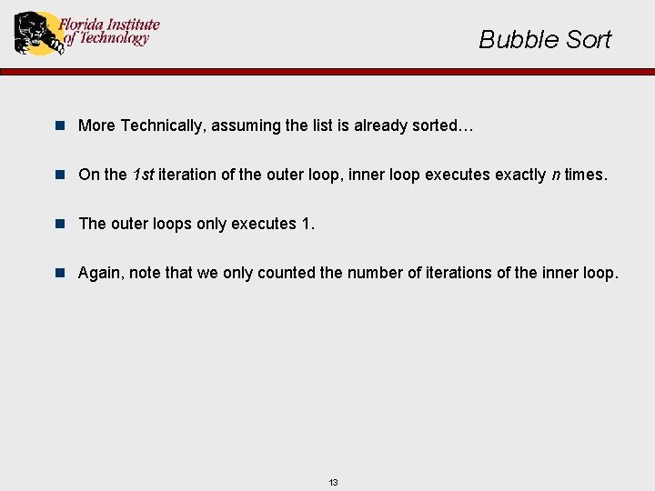
Bubble Sort n More Technically, assuming the list is already sorted… n On the 1 st iteration of the outer loop, inner loop executes exactly n times. n The outer loops only executes 1. n Again, note that we only counted the number of iterations of the inner loop. 13

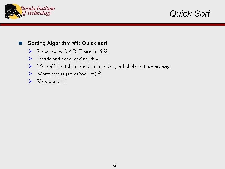
Quick Sort n Sorting Algorithm #4: Quick sort Ø Ø Ø Proposed by C. A. R. Hoare in 1962. Divide-and-conquer algorithm. More efficient than selection, insertion, or bubble sort, on average. Worst case is just as bad - Θ(n 2) Very practical. 14

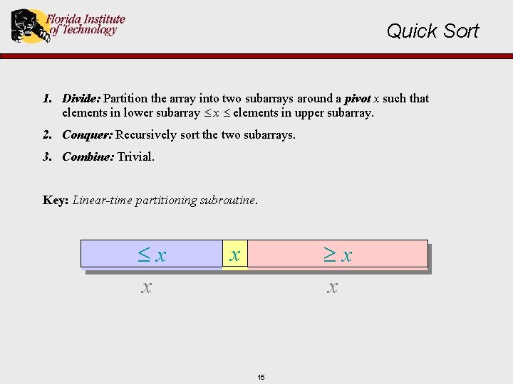
Quick Sort 1. Divide: Partition the array into two subarrays around a pivot x such that elements in lower subarray x elements in upper subarray. 2. Conquer: Recursively sort the two subarrays. 3. Combine: Trivial. Key: Linear-time partitioning subroutine. x ≤ x x ≥ x xx 15

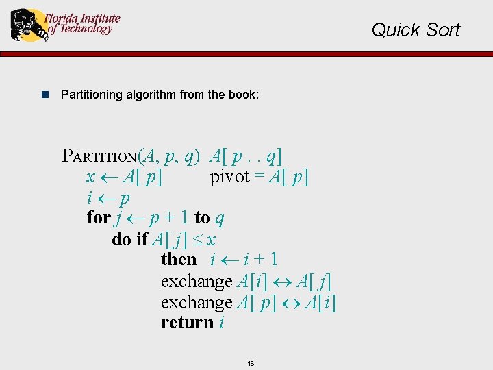
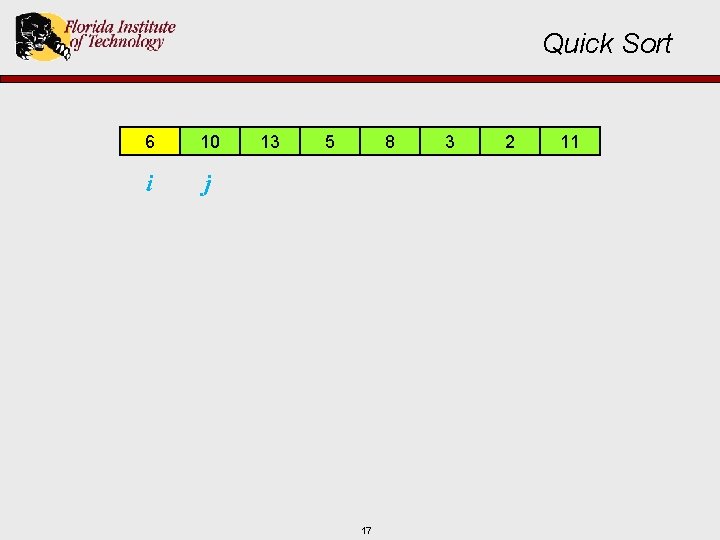
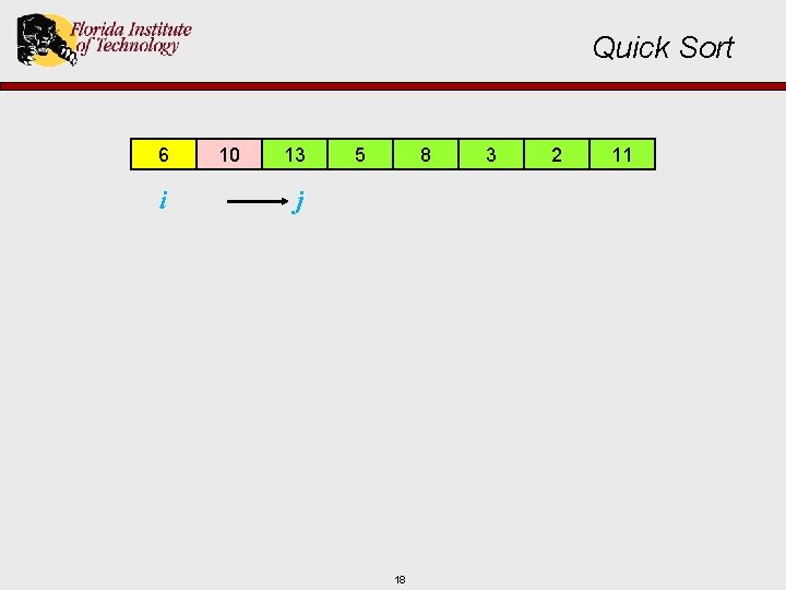
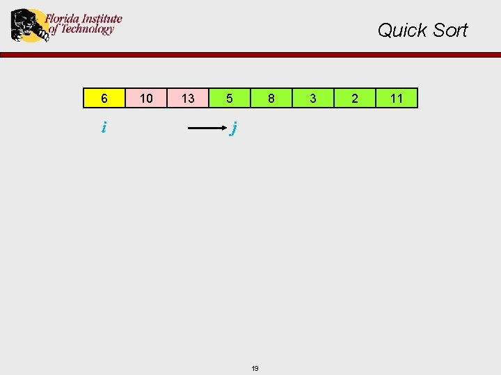
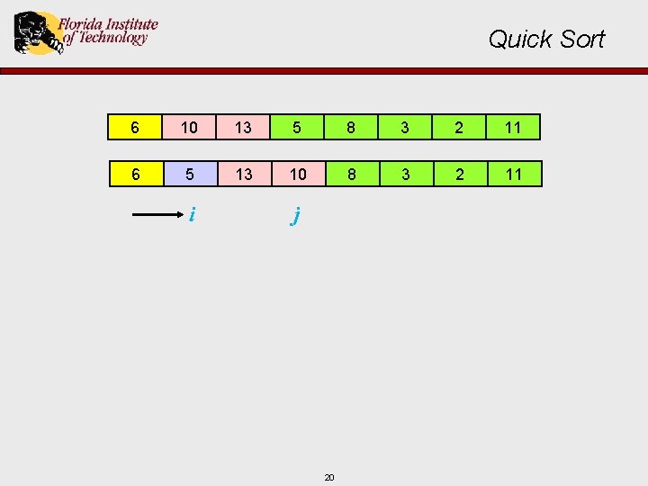
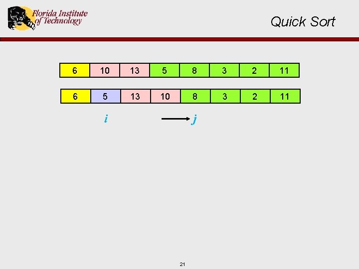
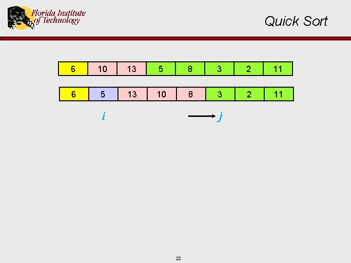
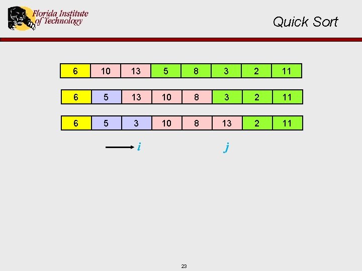
Quick Sort n Partitioning algorithm from the book: PARTITION(A, p, q) A[ p. . q] x A[ p] pivot = A[ p] i p for j p + 1 to q do if A[ j] x then i i + 1 exchange A[i] A[ j] exchange A[ p] A[i] return i 16

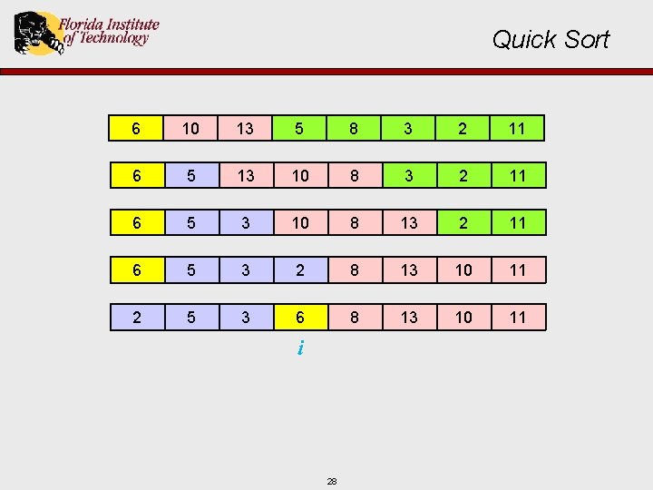
Quick Sort 6 10 i j 13 5 8 17 3 2 11

Quick Sort 6 i 10 13 5 8 j 18 3 2 11

Quick Sort 6 i 10 13 5 8 j 19 3 2 11

Quick Sort 6 10 13 5 8 3 2 11 6 5 13 10 8 3 2 11 i j 20

Quick Sort 6 10 13 5 8 3 2 11 6 5 13 10 8 3 2 11 j i 21

Quick Sort 6 10 13 5 8 3 2 11 6 5 13 10 8 3 2 11 j i 22

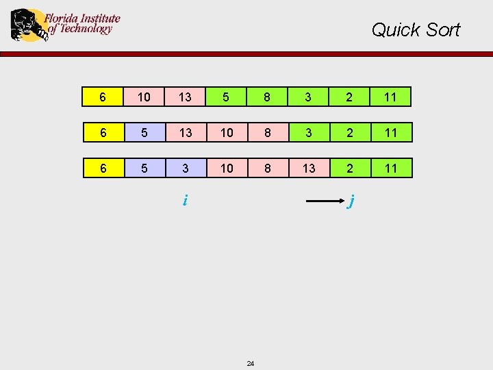
Quick Sort 6 10 13 5 8 3 2 11 6 5 13 10 8 3 2 11 6 5 3 10 8 13 2 11 i j 23

Quick Sort 6 10 13 5 8 3 2 11 6 5 13 10 8 3 2 11 6 5 3 10 8 13 2 11 i j 24

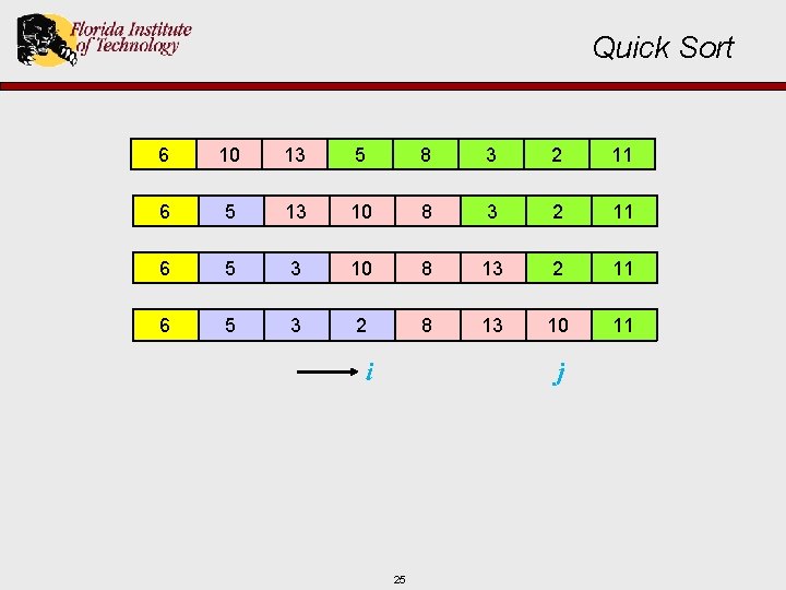
Quick Sort 6 10 13 5 8 3 2 11 6 5 13 10 8 3 2 11 6 5 3 10 8 13 2 11 6 5 3 2 8 13 10 11 i j 25

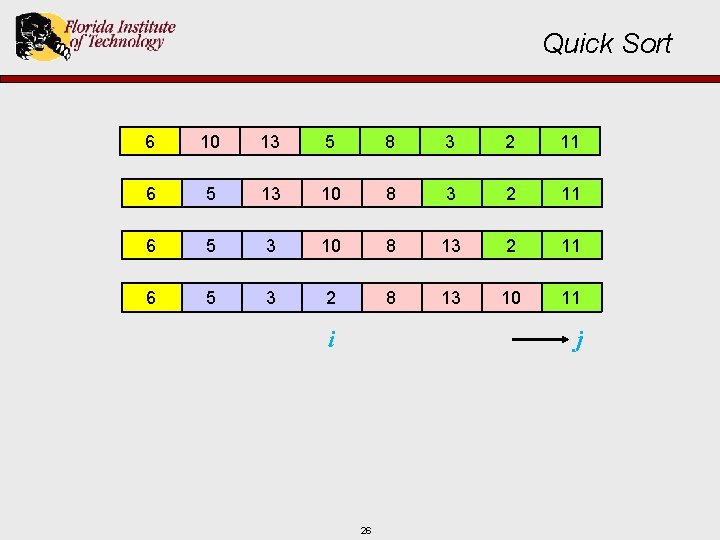
Quick Sort 6 10 13 5 8 3 2 11 6 5 13 10 8 3 2 11 6 5 3 10 8 13 2 11 6 5 3 2 8 13 10 11 i j 26

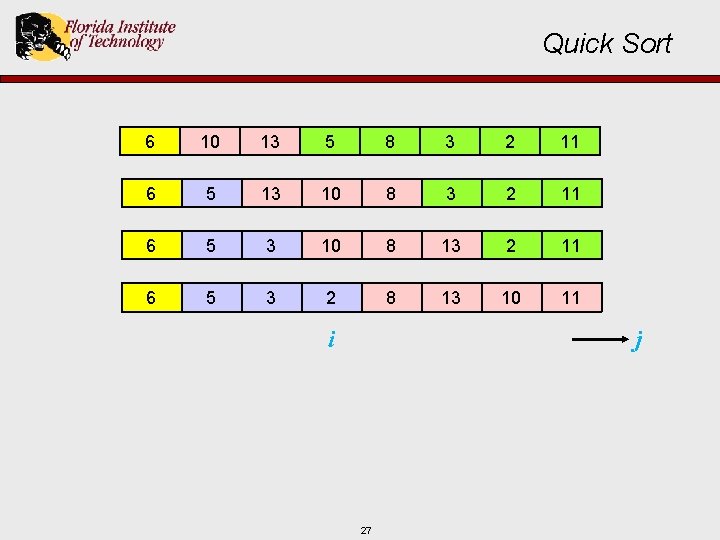
Quick Sort 6 10 13 5 8 3 2 11 6 5 13 10 8 3 2 11 6 5 3 10 8 13 2 11 6 5 3 2 8 13 10 11 i j 27

Quick Sort 6 10 13 5 8 3 2 11 6 5 13 10 8 3 2 11 6 5 3 10 8 13 2 11 6 5 3 2 8 13 10 11 2 5 3 6 8 13 10 11 i 28

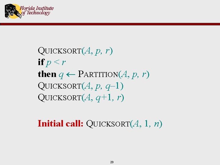
QUICKSORT(A, p, r) if p < r then q PARTITION(A, p, r) QUICKSORT(A, p, q– 1) QUICKSORT(A, q+1, r) Initial call: QUICKSORT(A, 1, n) 29

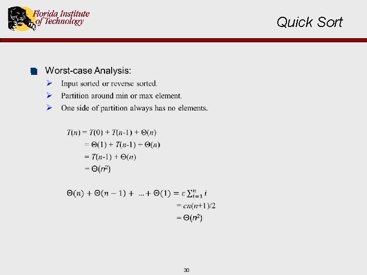
Quick Sort n 30

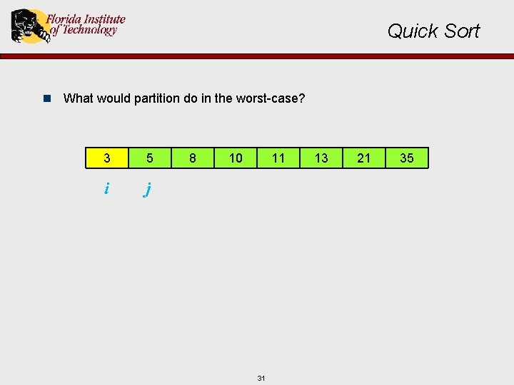
Quick Sort n What would partition do in the worst-case? 3 5 i j 8 10 11 31 13 21 35

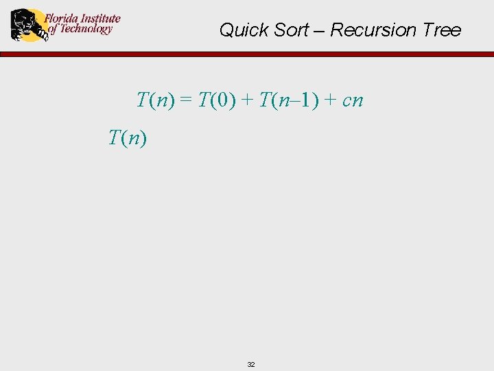
Quick Sort – Recursion Tree T(n) = T(0) + T(n– 1) + cn T(n) 32

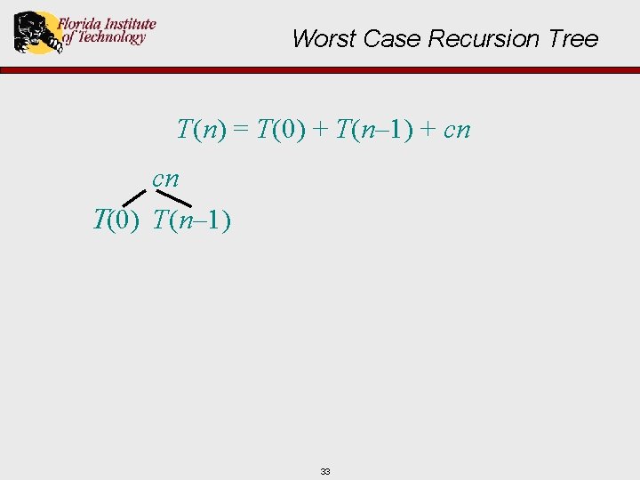
Worst Case Recursion Tree T(n) = T(0) + T(n– 1) + cn cn T(0) T(n– 1) 33

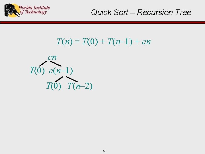
Quick Sort – Recursion Tree T(n) = T(0) + T(n– 1) + cn cn T(0) c(n– 1) T(0) T(n– 2) 34

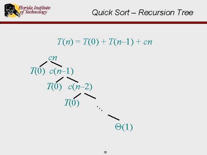
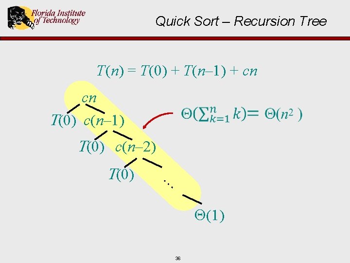
Quick Sort – Recursion Tree T(n) = T(0) + T(n– 1) + cn cn T(0) c(n– 1) T(0) c(n– 2) T(0) … (1) 35

Quick Sort – Recursion Tree T(n) = T(0) + T(n– 1) + cn cn T(0) c(n– 1) T(0) c(n– 2) T(0) … (1) 36

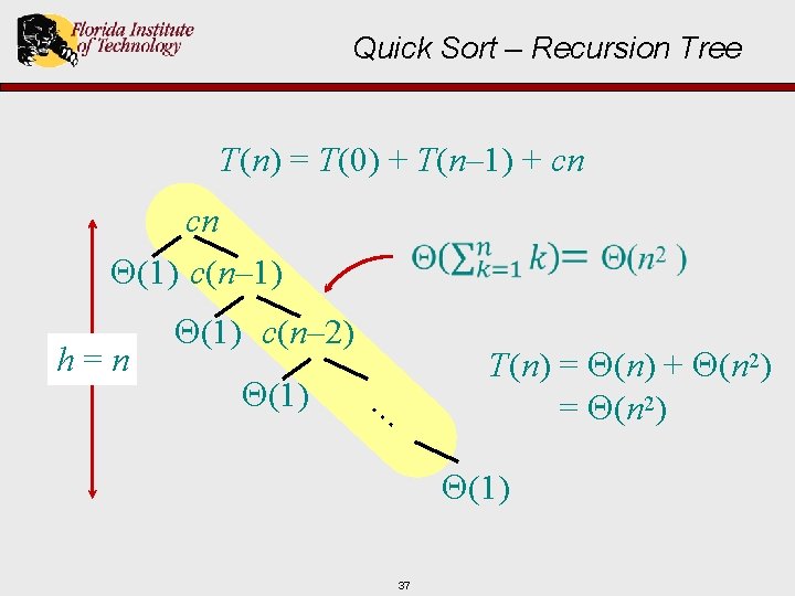
Quick Sort – Recursion Tree T(n) = T(0) + T(n– 1) + cn cn (1) c(n– 1) h = n (1) c(n– 2) (1) T(n) = (n) + (n 2) = (n 2) … (1) 37

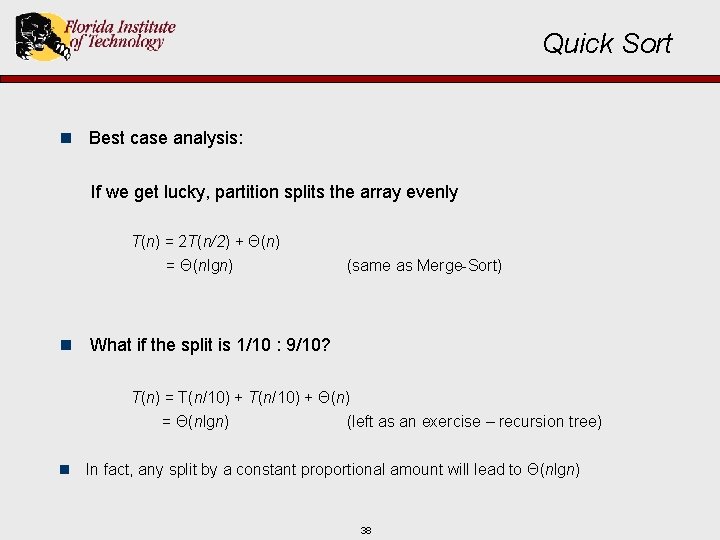
Quick Sort n Best case analysis: If we get lucky, partition splits the array evenly T(n) = 2 T(n/2) + Θ(n) = Θ(nlgn) (same as Merge-Sort) n What if the split is 1/10 : 9/10? T(n) = T(n/10) + Θ(n) = Θ(nlgn) (left as an exercise – recursion tree) n In fact, any split by a constant proportional amount will lead to Θ(nlgn) 38

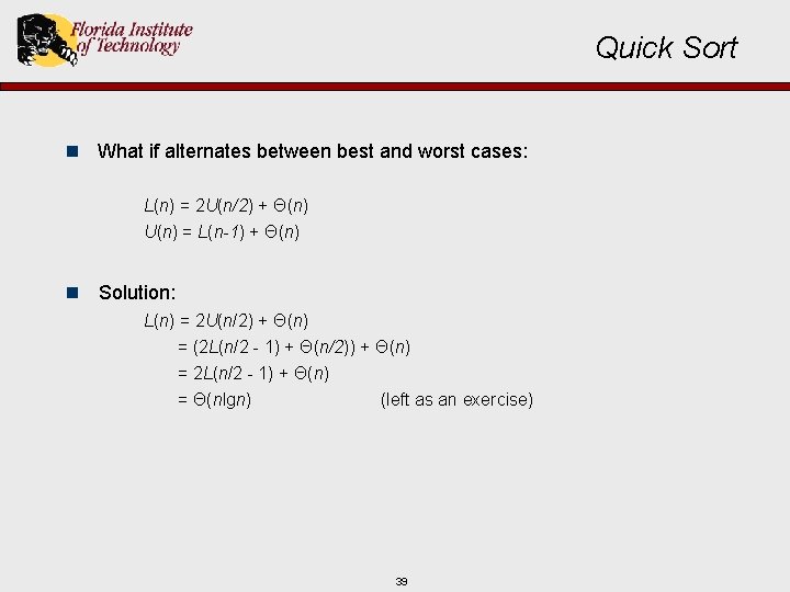
Quick Sort n What if alternates between best and worst cases: L(n) = 2 U(n/2) + Θ(n) U(n) = L(n-1) + Θ(n) n Solution: L(n) = 2 U(n/2) + Θ(n) = (2 L(n/2 - 1) + Θ(n/2)) + Θ(n) = 2 L(n/2 - 1) + Θ(n) = Θ(nlgn) (left as an exercise) 39

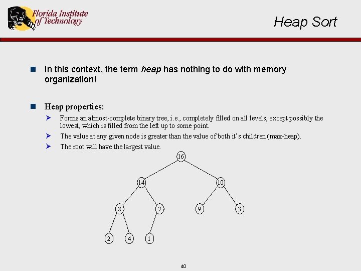
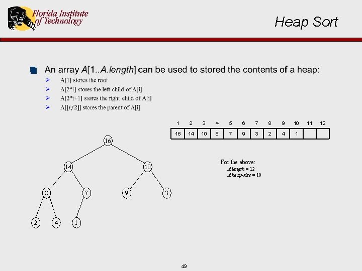
Heap Sort n In this context, the term heap has nothing to do with memory organization! n Heap properties: Ø Forms an almost-complete binary tree, i. e. , completely filled on all levels, except possibly the lowest, which is filled from the left up to some point. Ø Ø The value at any given node is greater than the value of both it’s children (max-heap). The root will have the largest value. 16 14 10 8 2 7 4 9 1 40 3

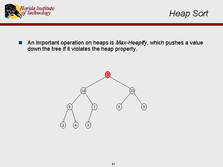
Heap Sort n An important operation on heaps is Max-Heapify, which pushes a value down the tree if it violates the heap property. 5 14 10 8 2 7 4 9 1 41 3

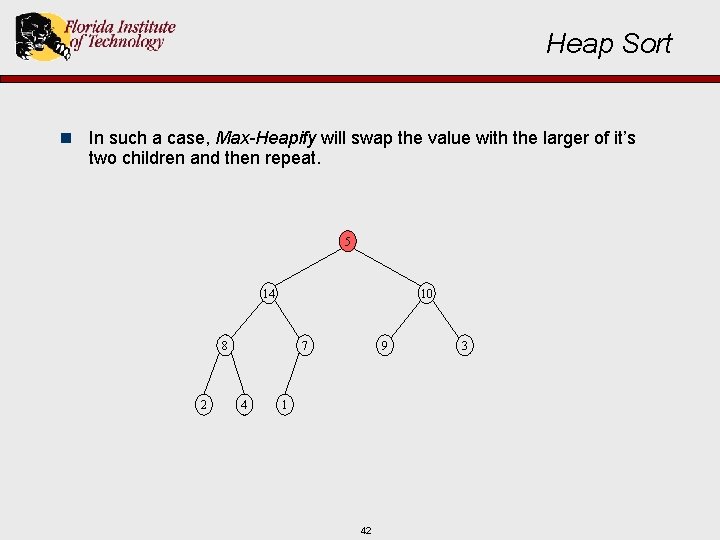
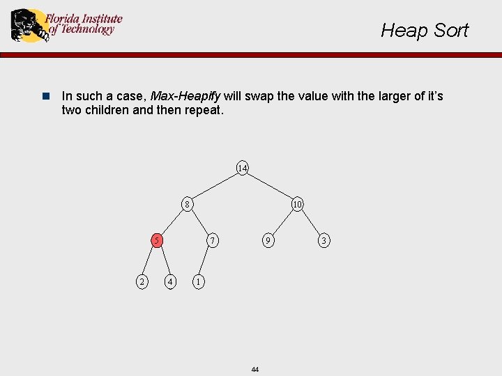
Heap Sort n In such a case, Max-Heapify will swap the value with the larger of it’s two children and then repeat. 5 14 10 8 2 7 4 9 1 42 3

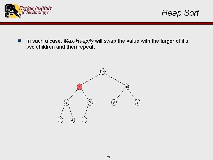
Heap Sort n In such a case, Max-Heapify will swap the value with the larger of it’s two children and then repeat. 14 10 5 8 2 7 4 9 1 43 3

Heap Sort n In such a case, Max-Heapify will swap the value with the larger of it’s two children and then repeat. 14 8 10 7 5 2 4 9 1 44 3

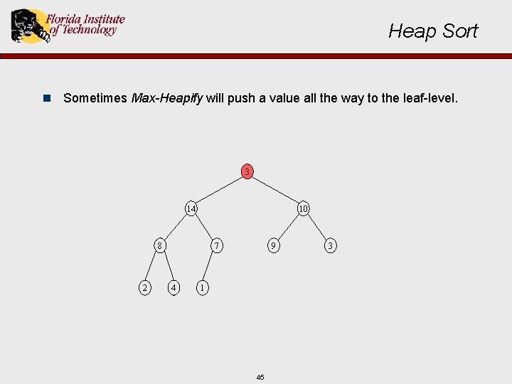
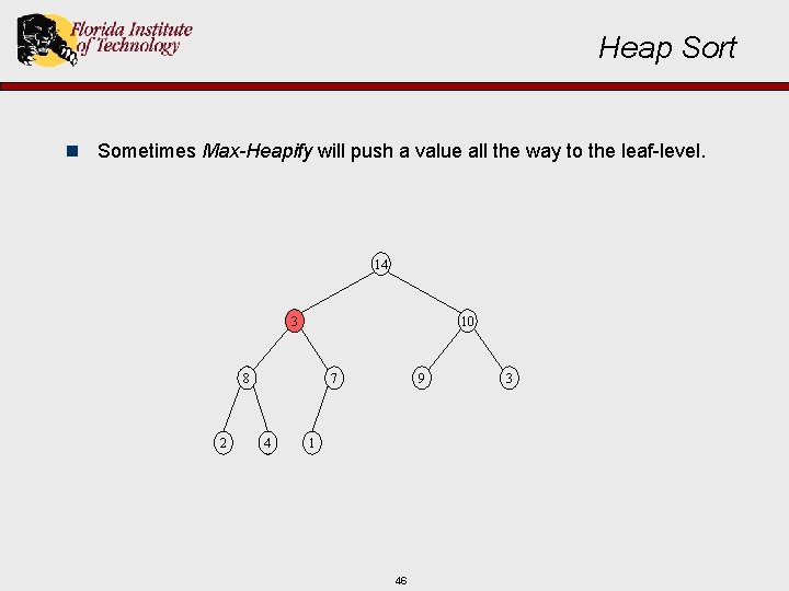
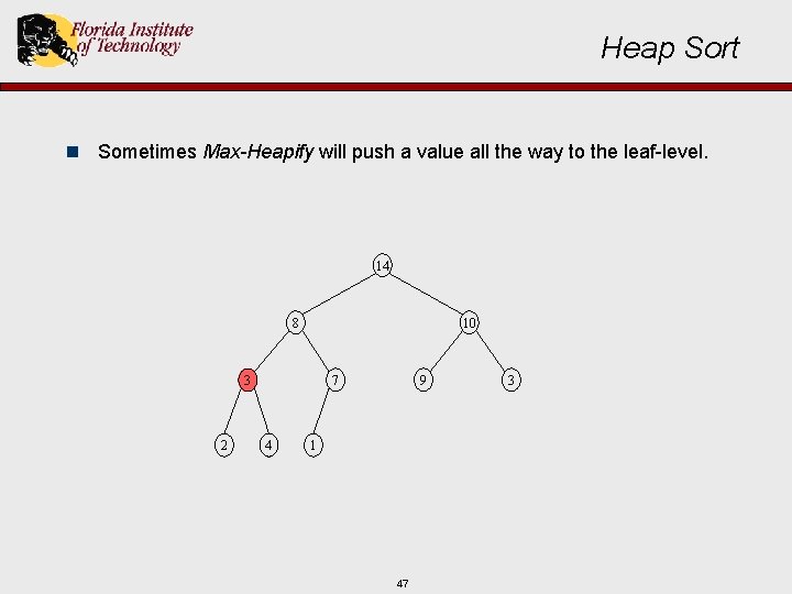
Heap Sort n Sometimes Max-Heapify will push a value all the way to the leaf-level. 3 14 10 8 2 7 4 9 1 45 3

Heap Sort n Sometimes Max-Heapify will push a value all the way to the leaf-level. 14 10 3 8 2 7 4 9 1 46 3

Heap Sort n Sometimes Max-Heapify will push a value all the way to the leaf-level. 14 8 10 7 3 2 4 9 1 47 3

Heap Sort n Sometimes Max-Heapify will push a value all the way to the leaf-level. 14 8 10 4 2 7 3 9 1 48 3

Heap Sort n 1 2 3 4 5 6 7 8 9 10 16 14 10 8 7 9 3 2 4 1 16 14 8 2 7 4 For the above: 10 9 A. length = 12 A. heap-size = 10 3 1 49 11 12

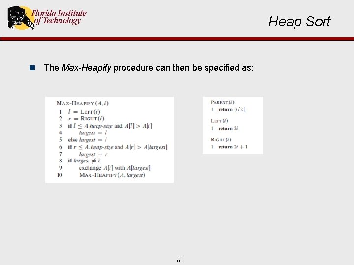
Heap Sort n The Max-Heapify procedure can then be specified as: 50

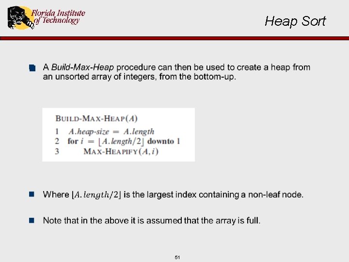
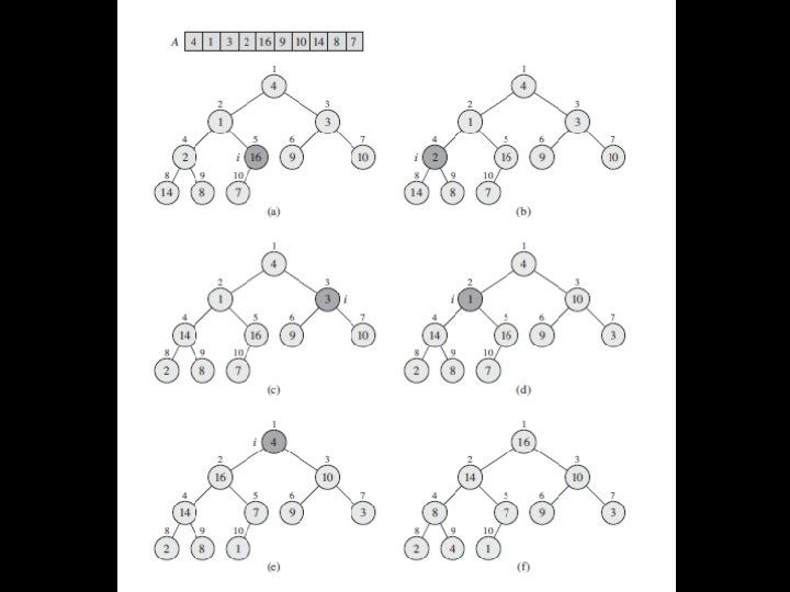
Heap Sort n 51

Heap Sort 52

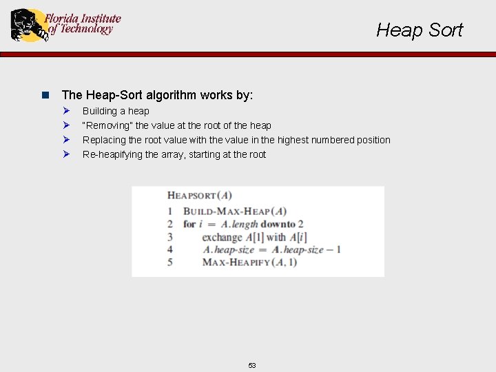
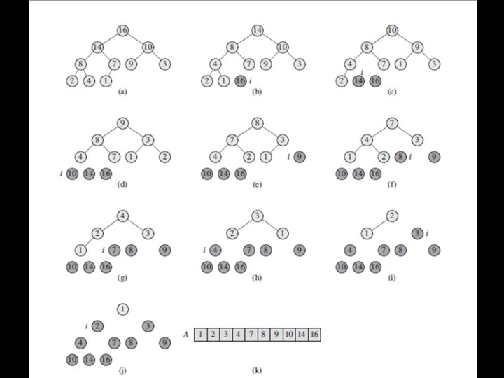
Heap Sort n The Heap-Sort algorithm works by: Ø Ø Building a heap “Removing” the value at the root of the heap Replacing the root value with the value in the highest numbered position Re-heapifying the array, starting at the root 53

Heap Sort 54

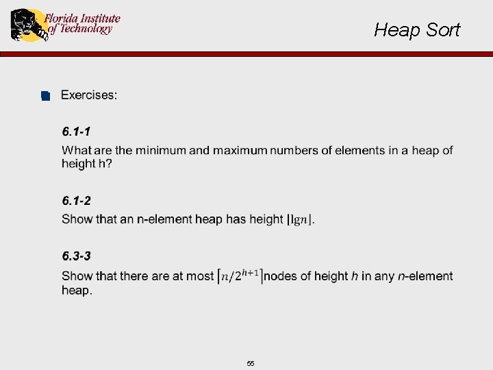
Heap Sort n 55

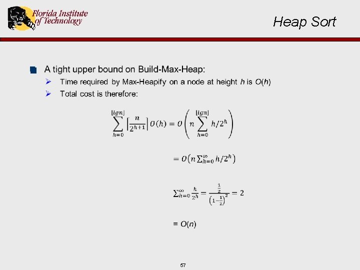
Heap Sort n Build-Max-Heap Analysis: Ø One call to Max-Heapify costs O(lgn) time. Ø Build-Max-Heap makes O(n) such calls. Ø Total is O(nlgn) cost. n This gives an upper-bound, but one that is not tight. 56

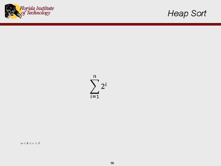
Heap Sort n 57

Heap Sort 58

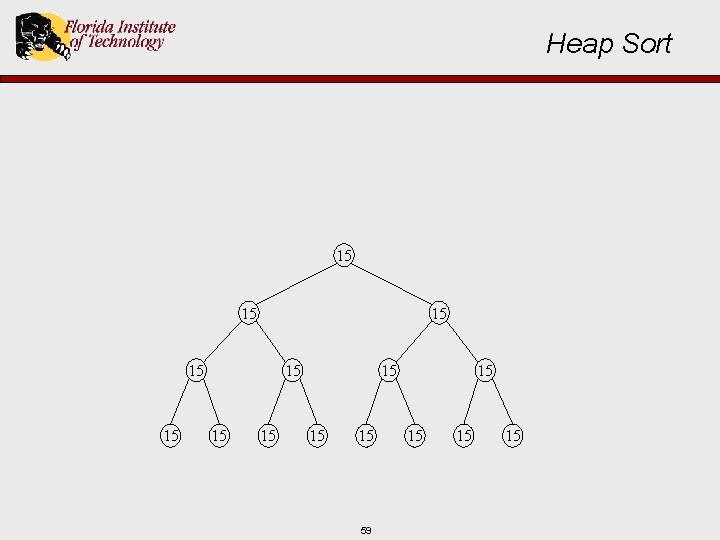
Heap Sort 15 15 15 59 15 15

How to Compare Algorithms in Efficiency n Empirical Analysis: Ø Experimentation: • Wall-clock time • CPU time • Requires many different inputs Ø Can you predict performance before implementing the algorithm? n Theoretical Analysis: Ø Approximation by counting important operations Ø Mathematical functions based on input size (N) 60

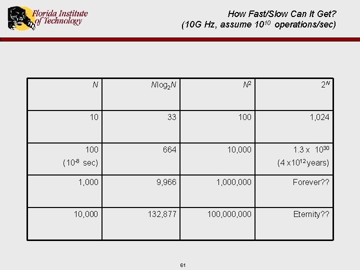
How Fast/Slow Can It Get? (10 G Hz, assume 1010 operations/sec) N Nlog 2 N N 2 2 N 10 33 100 1, 024 100 664 10, 000 1. 3 x 1030 (10 -8 sec) (4 x 1012 years) 1, 000 9, 966 1, 000 Forever? ? 10, 000 132, 877 100, 000 Eternity? ? 61