Patrick Royston MRC Clinical Trials Unit London UK

Patrick Royston MRC Clinical Trials Unit, London, UK Willi Sauerbrei Institut of Medical Biometry and Informatics University Medical Center Freiburg, Germany Use of FP and Other Flexible Methods to Assess Changes in the Impact of an exposure over time

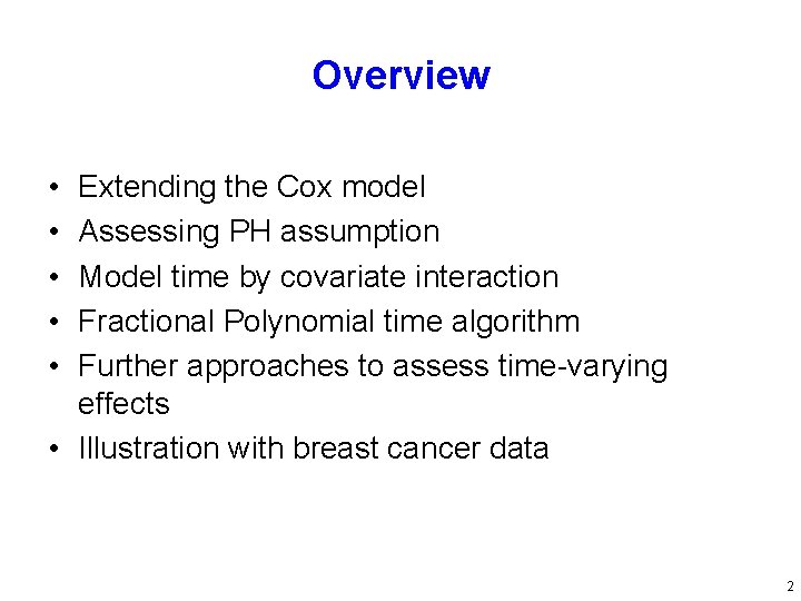
Overview • • • Extending the Cox model Assessing PH assumption Model time by covariate interaction Fractional Polynomial time algorithm Further approaches to assess time-varying effects • Illustration with breast cancer data 2

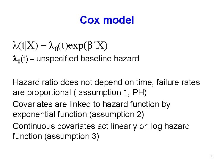
Cox model λ(t|X) = λ 0(t)exp(β΄X) 0(t) – unspecified baseline hazard Hazard ratio does not depend on time, failure rates are proportional ( assumption 1, PH) Covariates are linked to hazard function by exponential function (assumption 2) Continuous covariates act linearly on log hazard function (assumption 3) 3

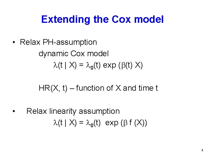
Extending the Cox model • Relax PH-assumption dynamic Cox model (t | X) = 0(t) exp ( (t) X) HR(X, t) – function of X and time t • Relax linearity assumption (t | X) = 0(t) exp ( f (X)) 4

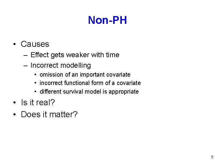
Non-PH • Causes – Effect gets weaker with time – Incorrect modelling • omission of an important covariate • incorrect functional form of a covariate • different survival model is appropriate • Is it real? • Does it matter? 5

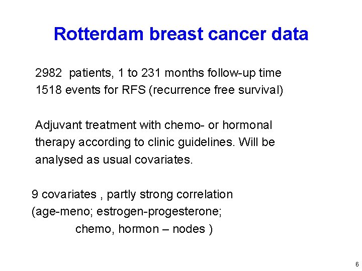
Rotterdam breast cancer data 2982 patients, 1 to 231 months follow-up time 1518 events for RFS (recurrence free survival) Adjuvant treatment with chemo- or hormonal therapy according to clinic guidelines. Will be analysed as usual covariates. 9 covariates , partly strong correlation (age-meno; estrogen-progesterone; chemo, hormon – nodes ) 6

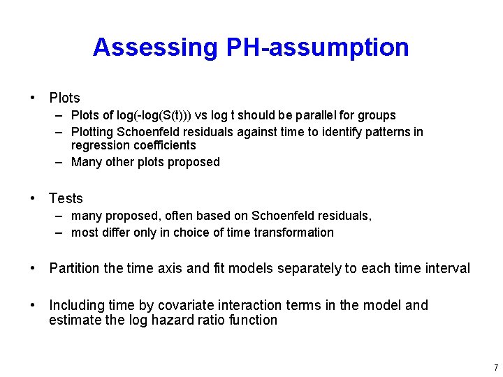
Assessing PH-assumption • Plots – Plots of log(-log(S(t))) vs log t should be parallel for groups – Plotting Schoenfeld residuals against time to identify patterns in regression coefficients – Many other plots proposed • Tests – many proposed, often based on Schoenfeld residuals, – most differ only in choice of time transformation • Partition the time axis and fit models separately to each time interval • Including time by covariate interaction terms in the model and estimate the log hazard ratio function 7

Smoothed Schoenfeld residuals - univariate models 8

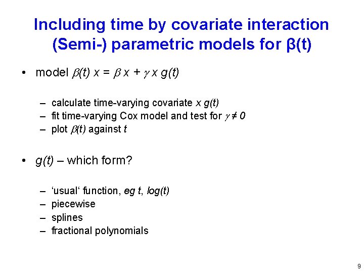
Including time by covariate interaction (Semi-) parametric models for β(t) • model (t) x = x + x g(t) – calculate time-varying covariate x g(t) – fit time-varying Cox model and test for ≠ 0 – plot (t) against t • g(t) – which form? – – ‘usual‘ function, eg t, log(t) piecewise splines fractional polynomials 9

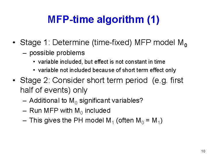
MFP-time algorithm (1) • Stage 1: Determine (time-fixed) MFP model M 0 – possible problems • variable included, but effect is not constant in time • variable not included because of short term effect only • Stage 2: Consider short term period (e. g. first half of events) only – Additional to M 0 significant variables? – Run MFP with M 0 included – This gives the PH model M 1 (often M 0 = M 1) 10

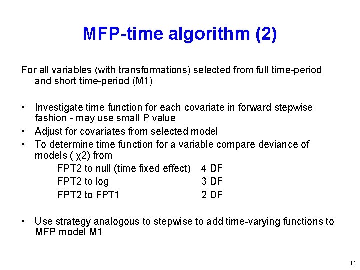
MFP-time algorithm (2) For all variables (with transformations) selected from full time-period and short time-period (M 1) • Investigate time function for each covariate in forward stepwise fashion - may use small P value • Adjust for covariates from selected model • To determine time function for a variable compare deviance of models ( χ2) from FPT 2 to null (time fixed effect) 4 DF FPT 2 to log 3 DF FPT 2 to FPT 1 2 DF • Use strategy analogous to stepwise to add time-varying functions to MFP model M 1 11

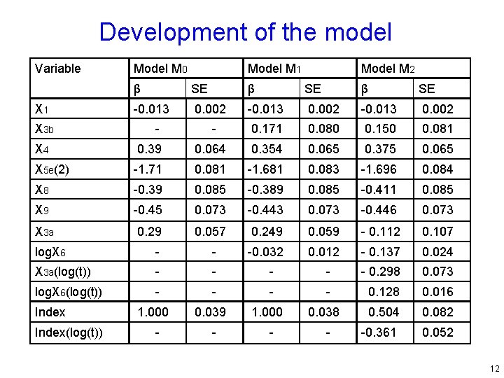
Development of the model Variable X 1 X 3 b Model M 0 Model M 1 Model M 2 β SE -0. 013 0. 002 0. 171 0. 080 0. 150 0. 081 - - X 4 0. 39 0. 064 0. 354 0. 065 0. 375 0. 065 X 5 e(2) -1. 71 0. 081 -1. 681 0. 083 -1. 696 0. 084 X 8 -0. 39 0. 085 -0. 389 0. 085 -0. 411 0. 085 X 9 -0. 45 0. 073 -0. 443 0. 073 -0. 446 0. 073 X 3 a 0. 29 0. 057 0. 249 0. 059 - 0. 112 0. 107 -0. 032 0. 012 - 0. 137 0. 024 log. X 6 - - X 3 a(log(t)) - - - 0. 298 0. 073 log. X 6(log(t)) - - 0. 128 0. 016 0. 504 0. 082 -0. 361 0. 052 Index(log(t)) 1. 000 - 0. 039 - 1. 000 - 0. 038 - 12

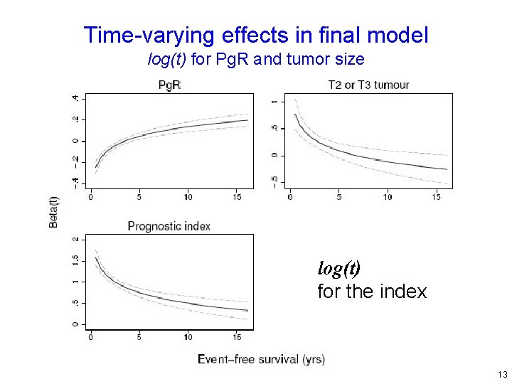
Time-varying effects in final model log(t) for Pg. R and tumor size log(t) for the index 13

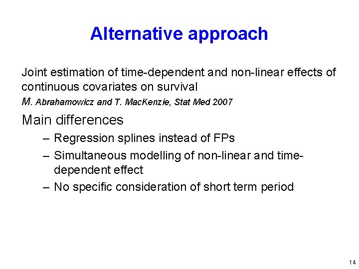
Alternative approach Joint estimation of time-dependent and non-linear effects of continuous covariates on survival M. Abrahamowicz and T. Mac. Kenzie, Stat Med 2007 Main differences – Regression splines instead of FPs – Simultaneous modelling of non-linear and timedependent effect – No specific consideration of short term period 14

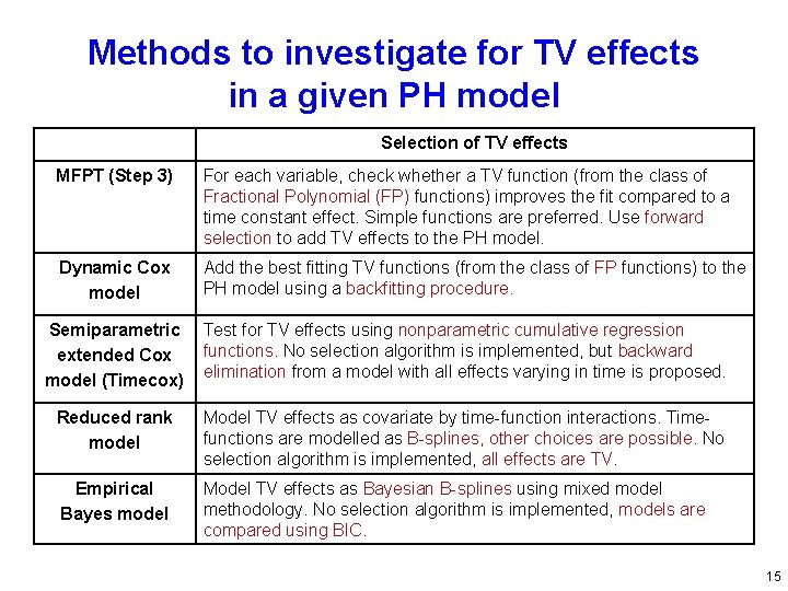
Methods to investigate for TV effects in a given PH model Selection of TV effects MFPT (Step 3) For each variable, check whether a TV function (from the class of Fractional Polynomial (FP) functions) improves the fit compared to a time constant effect. Simple functions are preferred. Use forward selection to add TV effects to the PH model. Dynamic Cox model Add the best fitting TV functions (from the class of FP functions) to the PH model using a backfitting procedure. Semiparametric extended Cox model (Timecox) Test for TV effects using nonparametric cumulative regression functions. No selection algorithm is implemented, but backward elimination from a model with all effects varying in time is proposed. Reduced rank model Model TV effects as covariate by time-function interactions. Timefunctions are modelled as B-splines, other choices are possible. No selection algorithm is implemented, all effects are TV. Empirical Bayes model Model TV effects as Bayesian B-splines using mixed model methodology. No selection algorithm is implemented, models are compared using BIC. 15

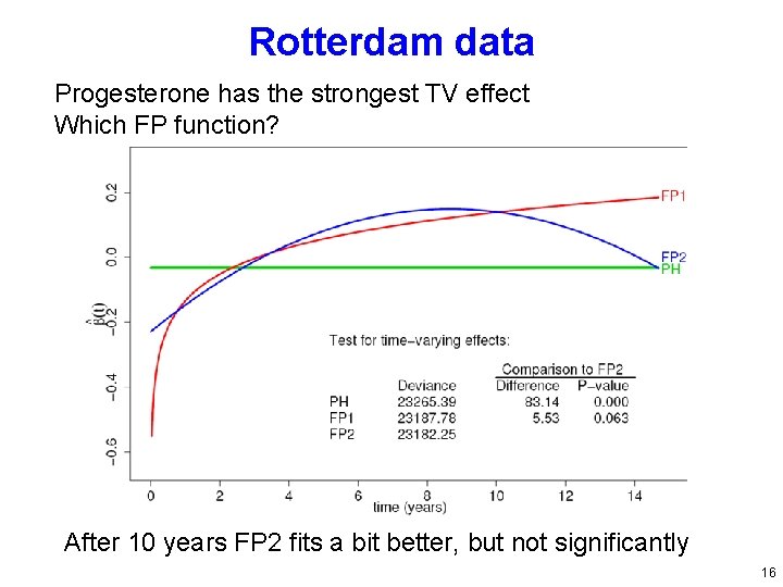
Rotterdam data Progesterone has the strongest TV effect Which FP function? After 10 years FP 2 fits a bit better, but not significantly 16

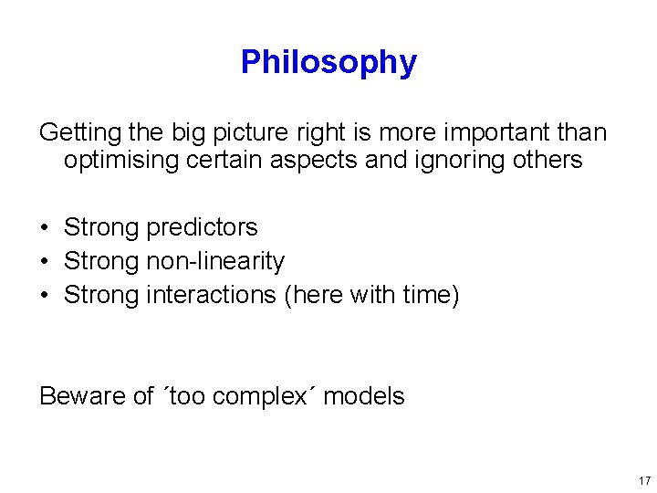
Philosophy Getting the big picture right is more important than optimising certain aspects and ignoring others • Strong predictors • Strong non-linearity • Strong interactions (here with time) Beware of ´too complex´ models 17

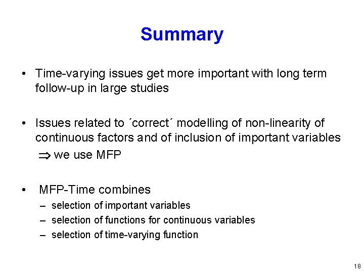
Summary • Time-varying issues get more important with long term follow-up in large studies • Issues related to ´correct´ modelling of non-linearity of continuous factors and of inclusion of important variables we use MFP • MFP-Time combines – selection of important variables – selection of functions for continuous variables – selection of time-varying function 18

Summary (continued) • Further extension of MFP – Interaction of a continuous variable with treatment or between two continuous variables • Our FP based approach is simple, but needs ´fine tuning´ and investigation of properties • Comparison to other approaches is required 19

References - FP methodology Royston P, Altman DG. (1994): Regression using fractional polynomials of continuous covariates: parsimonious parametric modelling (with discussion). Applied Statistics, 43, 429 -467. Royston P, Altman DG, Sauerbrei W. (2006): Dichotomizing continuous predictors in multiple regression: a bad idea. Statistics in Medicine, 25: 127 -141. Royston P, Sauerbrei W. (2005): Building multivariable regression models with continuous covariates, with a practical emphasis on fractional polynomials and applications in clinical epidemiology. Methods of Information in Medicine, 44, 561 -571. Royston P, Sauerbrei W. (2008): Interactions between treatment and continuous covariates – a step towards individualizing therapy (Editorial). JCO, 26: 1397 -1399. Royston P, Sauerbrei W. (2008): Multivariable Model-Building - A pragmatic approach to regression analysis based on fractional polynomials for modelling continuous variables. Wiley. Sauerbrei W, Royston P. (1999): Building multivariable prognostic and diagnostic models: transformation of the predictors by using fractional polynomials. Journal of the Royal Statistical Society A, 162, 71 -94. Sauerbrei, W. , Royston, P. , Binder H (2007): Selection of important variables and determination of functional form for continuous predictors in multivariable model building. Statistics in Medicine, to appear Sauerbrei W, Royston P, Look M. (2007): A new proposal for multivariable modelling of time-varying effects in survival data based on fractional polynomial timetransformation. Biometrical Journal, 49: 453 -473. 20

References – Time-varying effects Abrahamovicz M, Mac. Kenzie TA. (2007): Joint estimation of time-dependent and nonlinear effects of continuous covariates on survival. Statistics in Medicine. Berger U, Schäfer J, Ulm K. (2003): Dynamic Cox modelling based on fractional polynomials: time-variations in gastric cancer prognosis. Statistics in Medicine, 22: 1163– 1180 Kneib T, Fahrmeir L. (2007): Amixedmodel approach for geoadditive hazard regression. Scandinavian Journal of Statistics, 34: 207– 228. Perperoglou A, le Cessie S, van Houwelingen HC. (2006): Reduced-rank hazard regression for modelling non-proportional hazards. Statistics in Medicine, 25: 2831– 2845. Sauerbrei W, Royston P, Look M. (2007): A new proposal for multivariable modelling of timevarying effects in survival data based on fractional polynomial timetransformation. Biometrical Journal, 49: 453– 473. Scheike T H, Martinussen T. (2004): On estimation and tests of time-varying effects in the proportionalhazards model. Scandinavian Journal of Statistics, 31: 51– 62. 21