Overview of the RHtestsdly Prcp software package for

Overview of the RHtests_dly. Prcp software package for homogenization of daily precipitation Xiaolan L. Wang and Y. Feng Climate Research Division, Science & Technology Branch, Environment Cana EMS 2015, Sofia, Bulgaria, 7 -11 September 2015

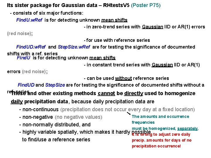
Its sister package for Gaussian data – RHtests. V 5 (Poster P 75) - consists of six major functions: Find. U. w. Ref is for detecting unknown mean shifts - in zero-trend series with Gaussian IID or AR(1) errors (red noise); - for use with reference series Find. UD. w. Ref and Step. Size. w. Ref are for testing the significance of documented shifts with a ref. series Find. U is for detecting unknown mean shifts - in constant trend series with Gaussian IID or AR(1) errors (red noise); - can be used without reference series Find. UD and Step. Size are for testing the significance of documented shifts without a ref. seriesand other existing methods cannot be directly used to homogenize These daily precipitation data, because daily precipitation data are - non-continuous (precipitation does not occur every day at a fixed location) The amounts and occurrence - non-negative (no negative values) frequencies - non-normally distributed, and must be homogenized, separately. - highly variable spatially, which makes it hardly possible It is wrong to adjust zero daily to find/use a reference series precip. amounts for days of no precipitation occurrence!

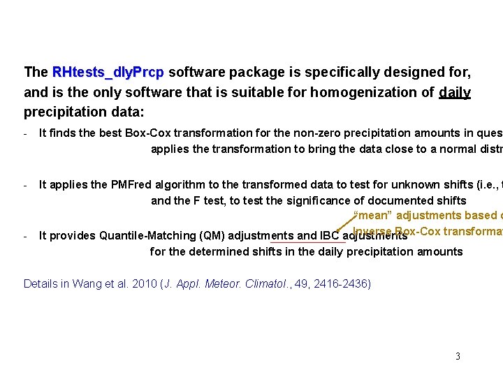
The RHtests_dly. Prcp software package is specifically designed for, and is the only software that is suitable for homogenization of daily precipitation data: - It finds the best Box-Cox transformation for the non-zero precipitation amounts in quest applies the transformation to bring the data close to a normal distr - It applies the PMFred algorithm to the transformed data to test for unknown shifts (i. e. , t and the F test, to test the significance of documented shifts “mean” adjustments based o Inverse Box-Cox transformat It provides Quantile-Matching (QM) adjustments and IBC adjustments - for the determined shifts in the daily precipitation amounts Details in Wang et al. 2010 (J. Appl. Meteor. Climatol. , 49, 2416 -2436) 3

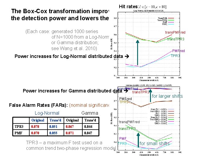
Hit rates: The Box-Cox transformation improves Log-Normal data the detection power and lowers the FAR (Each case: generated 1000 series of N=1000 from a Log-Normal or Gamma distribution; see Wang et al. 2010) trans. PMFred trans. TPR 3 PMFred TPR 3 Power increases for Log-Normal distributed data trans. PMFred Power increases for Gamma distributed data trans. TPR 3 PMFred TPR 3 for larger shifts False Alarm Rates (FARs): (nominal significance: 0. 05) Log-Normal Gamma Original Trans’d TPR 3 0. 078 0. 051 0. 067 0. 044 PMF 0. 070 0. 055 0. 071 0. 047 TPR 3 – a maximum F test used on a common trend two-phase regression model trans. PMFred trans. TPR 3 PMF TPR 3 for small shifts

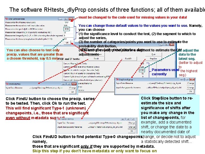
The software RHtests_dly. Prcp consists of three functions; all of them available must be changed to the code used for missing values in your data! You can also choose to test only precip. values that are greater than a chosen threshold, say 0. 5 mm You can change these default values to the values you want to use. Namely, you can choose (1) the significance level to conduct the test, (2) the segment to which to adjust the series, (3) the number of categories/points you want to use to estimate the probability distribution, (4) to use all or part of the data in a segment to estimate the QM to adjust the adjustments data to the latest seg. (better to adjust to Parameters used the highest currently seg. ) Click Step. Size button to reestimate the size and significance of shifts after you make any change in the list of changepoints, for example, add a documented shift, or change the date to a nearby documented date of change, or decide not to adjust Click Find. UD button to find potential Type-0 changepoints, a statistically detected shift… namely, those that are significant only if they are supported by metadata. Skip this step if you don’t have metadata or only want to focus on Click Find. U button to choose the precip. series to be tested. Then, click Ok to run the test. This will find significant Type-1 (unknown) changepoints, i. e. , those that are significant even without metadata support

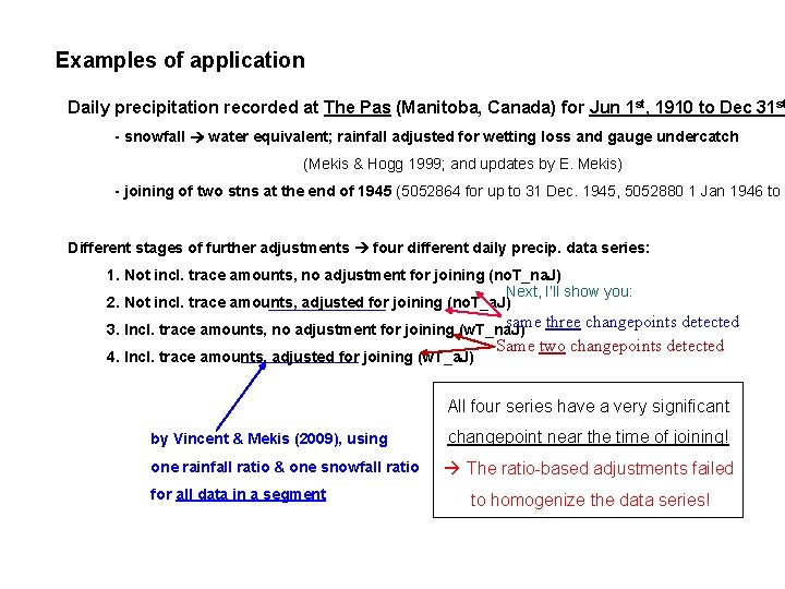
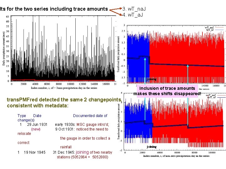
Examples of application Daily precipitation recorded at The Pas (Manitoba, Canada) for Jun 1 st, 1910 to Dec 31 st - snowfall water equivalent; rainfall adjusted for wetting loss and gauge undercatch (Mekis & Hogg 1999; and updates by E. Mekis) - joining of two stns at the end of 1945 (5052864 for up to 31 Dec. 1945, 5052880 1 Jan 1946 to 3 Different stages of further adjustments four different daily precip. data series: 1. Not incl. trace amounts, no adjustment for joining (no. T_na. J) Next, I’ll show you: 2. Not incl. trace amounts, adjusted for joining (no. T_a. J) same three changepoints detected Same two changepoints detected 3. Incl. trace amounts, no adjustment for joining (w. T_na. J) 4. Incl. trace amounts, adjusted for joining (w. T_a. J) All four series have a very significant by Vincent & Mekis (2009), using one rainfall ratio & one snowfall ratio for all data in a segment changepoint near the time of joining! à The ratio-based adjustments failed to homogenize the data series!

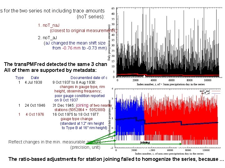
no. T_na. J ts for the two series not including trace amounts (no. T series): 1. no. T_na. J (closest to original measurements): 2. no. T_a. J (a. J changed the mean shift size from -0. 76 mm to -0. 73 mm) The trans. PMFred detected the same 3 changepoints. All of them are supported by metadata: Type Date 1 4 Jul 1938 1 24 Oct 1946 1 4 Oct 1976 Documented date of change(s) 9 Oct 1937 to 8 Aug 1938: changes in gauge type, rim height, observing frequency; poor gauge condition reported on 9 Oct 1937 31 Dec 1945: joining of two nearby stations (5052864 + 5052880) 16 Oct 1975 to 18 Oct 1977: gauge type change (standard at 12” rim height to Type B at 16” rim height) Reflect changes in the min. measurable amount (precision, unit) -0. 76 mm 1937 -38 joining 1945 -46 joining 1976 -77 The ratio-based adjustments for station joining failed to homogenize the series, because …

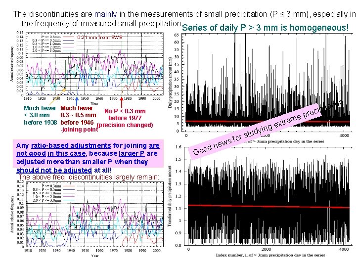
The discontinuities are mainly in the measurements of small precipitation (P ≤ 3 mm), especially in the frequency of measured small precipitation: Series of daily P > 3 mm is homogeneous! 0. 21 mm from SWE no. T_na. J > 3 mm no. T_na. J Much fewer No P < 0. 3 mm < 3. 0 mm 0. 3 ~ 0. 5 mm before 1977 before 1938 before 1946 (precision changed) -joining point Any ratio-based adjustments for joining are not good in this case, because larger P are adjusted more than smaller P when they should not be adjusted at all! The above freq. discontinuities largely remain: no. T_a. J xtr e g n yi s Go ew od n tud for s em ipita c e r ep no. T_na. J > 3 mm tion

lts for the two series including trace amounts 3. w. T_na. J 4. w. T_a. J w. T_na. J joining Inclusion of trace amounts makes these shifts disappeared! trans. PMFred detected the same 2 changepoints, consistent with metadata: Type Date change(s) 1 29 Jun 1931 (new) relocate Documented date of early 1930 s: MSC gauge intro’d; 9 Oct 1931: noticed the need to the gauge in order to collect a correct 1 19 Nov 1945 rainfall 31 Dec 1945: joining of two nearby stations (5052864 + 5052880) 1937 -38 joining 1976 -77

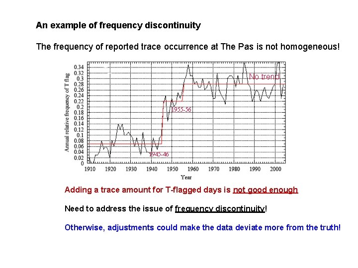
An example of frequency discontinuity The frequency of reported trace occurrence at The Pas is not homogeneous! no. T_na. J No trend 1955 -56 1945 -46 Adding a trace amount for T-flagged days is not good enough Need to address the issue of frequency discontinuity! Otherwise, adjustments could make the data deviate more from the truth!

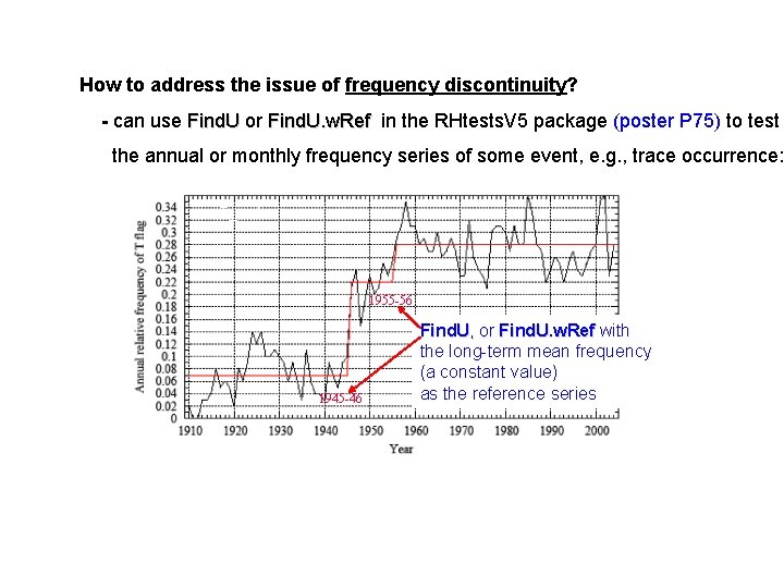
How to address the issue of frequency discontinuity? - can use Find. U or Find. U. w. Ref in the RHtests. V 5 package (poster P 75) to test the annual or monthly frequency series of some event, e. g. , trace occurrence: no. T_na. J 1955 -56 1945 -46 Find. U, or Find. U. w. Ref with the long-term mean frequency (a constant value) as the reference series

Concluding remarks - Homogenization of daily precipitation data is very challenging Recommend: test series of daily. P > Pthr with different Pthr values (e. g. , 0. 0, 0. 3 mm, 0. 5 mm, 1. 0 mm) should be chosen to reflect changes in measurement precision/unit also check the frequency series of small P, because small P are harder to measure with accuracy than larger P (larger %e – discontinuities often exist in freq series of small P (e. g. P < 0. 5 m In the presence of frequency discontinuity, any adjustment derived from the measured daily P is not good. (e. g. , ratio-based, IBC, Quantile-Matching) One must address the issue of freq. discontinuity first! Shall aim to get better insight into the cause (metadata) and characteristics of disco (e. g. , freq. ) before any attempt to adjust daily precipitation data – a non-continuous

The package is available at http: //etccdi. pacificclimate. org/software. shtml Thank you very much for your attention! Questions/comments?