Microeconomics Corso E John Hey Summary of Chapter

Microeconomics Corso E John Hey

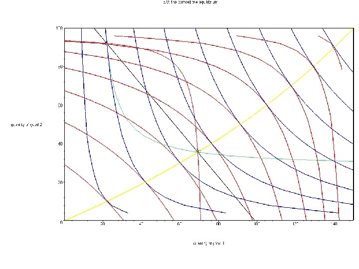
Summary of Chapter 8 • The contract curve shows the allocations that are efficient in the sense of Pareto. • There always exist the possibility of mutually advantageous exchange if preferences are different and/or endowments are different (unless the endowment point is on the contract curve). • Perfect competitive equilibrium (with both individuals taking the price as given) always leads to a Pareto efficient allocation. • If one of the individuals chooses the price the allocation is not Pareto efficient.

The competitive equilibrium depends on the preferences and the endowments. • If one individual changes his or her preferences in such a way that he or she now prefers more a particular good than before. . . • . . . the relative price of that good rises. • If an individual is endowed with more of a good than before. . . • . . . the relative price of that good falls.

Part 1 and Part 2 • Part 1: an economy without production. . . • . . . just exchange • Part 2: an economy with production. . . • . . . production and exchange.

Part 1 • • • Reservation prices. Indifference curves. Demand supply curves. Surplus. Exchange. The Edgeworth Box. The contract curve. Competitive equilibrium. Paretian efficiency and inefficiency.

Part 2 • Chapter 10: Technology. • Chapter 11: Minimisation of costs and factor demands. • Chapter 12: Cost curves. • Chapter 13: Firm’s supply and profit/surplus. • Chapter 14: The production possibility frontier. • Chapter 15: Production and exchange.

Chapter 10 • • Firms produce. . . they use inputs to produce outputs. In general many inputs and many outputs. We work with a simple firm that produces one output with two inputs. . . • . . . capital and labour. • The technology describes the possibilities open to the firm.

Chapter 5 • Individuals • Buy goods and ‘produce’ utility… • …depends on the preferences… • …which we can represent with indifference curves. . • …in the space (q 1, q 2) Chapter 10 • Firms • Buy inputs and produce output… • …depends on the technology… • …which we can represent with isoquants. . • …in the space (q 1, q 2)

The only difference? • We can represent preferences with a utility function. . . • . . . but this function is not unique. . . • . . . because/hence we cannot measure the utility of an individual. • We can represent the technology of a firm with a production function. . . • . . . and this function is unique… • …because we can measure the output.

An isoquant • In the space of the inputs (q 1, q 2) it is the locus of the points where output is constant. • (An indifference curve – the locus of the points where the individual is indifferent. Or the locus of points for which the utility is constant. )

Two dimensions • The shape of the isoquants: depends on the substitution between the two inputs. • The way in which the output changes form one isoquant to another – depends on the returns to scale.

Perfect substitutes 1: 1 • an isoquant: q 1 + q 2 = constant • y = A(q 1 + q 2) constant returns to scale • y = A(q 1 + q 2)0. 5 decreasing returns to scale • y = A(q 1 + q 2)2 increasing returns to scale • y = A(q 1 + q 2)b returns to scale decreasing (b<1) increasing (b>1)

y = q 1 + q 2 : perfect substitutes 1: 1 and constant returns to scale

y = (q 1 + q 2)2 : perfect substitutes 1: 1 and increasing returns to scale

y = (q 1 + q 2)0. 5 : perfect substitutes 1: 1 and decreasing returns to scale

Perfect Substitutes 1: a • an isoquant: q 1 + q 2/a = constant • y = A(q 1 + q 2/a) constant returns to scale • y = A(q 1 + q 2/a)b returns to scale decreasing (b<1) increasing (b>1)

Perfect Complements 1 with 1 • an isoquant: min(q 1, q 2) = constant • y = A min(q 1, q 2) constant returns to scale • y = A[min(q 1, q 2)]b returns to scale decreasing (b<1) increasing (b>1)

y = min(q 1, q 2): Perfect Complements 1 with 1 and constant returns to scale

y = [min(q 1, q 2)]2 Perfect Complements 1 with 1 and increasing returns to scale

Y = [min(q 1, q 2)]0. 5: Perfect Complements 1 with 1 and decreasing returns to scale

Perfect Complements 1 with a • an isoquant: min(q 1, q 2/a) = constant • y = A min(q 1, q 2/a) constant returns to scale • y = A[min(q 1, q 2/a)]b returns to scale decreasing (b<1) increasing (b>1)

y = q 10. 5 q 20. 5: Cobb-Douglas with parameters 0. 5 and 0. 5 – hence constant returns to scale

y = q 1 q 2: Cobb-Douglas with parameters 1 and 1 – hence increasing returns to scale

y = q 10. 25 q 20. 25: Cobb-Douglas with parameters 0. 25 and 0. 25 – hence decreasing returns to scale

Cobb-Douglas with parameters a and b • an isoquant: q 1 a q 2 b = constant • y = A q 1 a q 2 b • a+b<1 decreasing returns to scale • a+b=1 constant returns to scale • a+b>1 increasing returns to scale

Chapter 5 • Individuals • The preferences are given by indifference curves • …in the space (q 1, q 2) • . . can be represented by a utility function u = f(q 1, q 2)… • …which is not unique. Chapter 10 • Firms • The technology is given by isoquants • …in the space (q 1, q 2) • . . can be represented by a production function … y = f(q 1, q 2)… • … which is unique.

Chapter 10 • Goodbye!