Markov Chain Monte Carlo Gil Mc Vean Tuesday

Markov Chain Monte Carlo Gil Mc. Vean Tuesday 24 th February 2009 1

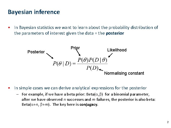
Bayesian inference • In Bayesian statistics we want to learn about the probability distribution of the parameters of interest given the data = the posterior Prior Likelihood Normalising constant • In simple cases we can derive analytical expressions for the posterior – For example, if we have a beta prior: Beta(a, b) for a binomial parameter, after we have observed n successes and m failures, the posterior is also beta: Beta(a+n, b+m). The key here is conjugacy. 2

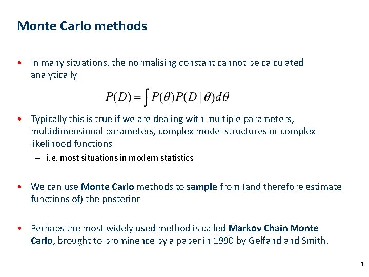
Monte Carlo methods • In many situations, the normalising constant cannot be calculated analytically • Typically this is true if we are dealing with multiple parameters, multidimensional parameters, complex model structures or complex likelihood functions – i. e. most situations in modern statistics • We can use Monte Carlo methods to sample from (and therefore estimate functions of) the posterior • Perhaps the most widely used method is called Markov Chain Monte Carlo, brought to prominence by a paper in 1990 by Gelfand Smith. 3

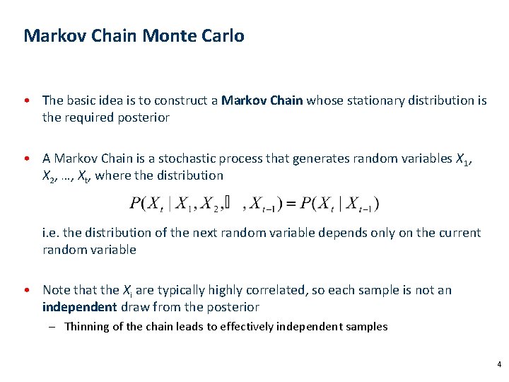
Markov Chain Monte Carlo • The basic idea is to construct a Markov Chain whose stationary distribution is the required posterior • A Markov Chain is a stochastic process that generates random variables X 1, X 2, …, Xt, where the distribution i. e. the distribution of the next random variable depends only on the current random variable • Note that the Xi are typically highly correlated, so each sample is not an independent draw from the posterior – Thinning of the chain leads to effectively independent samples 4

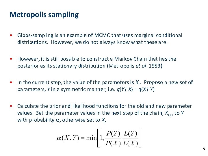
Metropolis sampling • Gibbs-sampling is an example of MCMC that uses marginal conditional distributions. However, we do not always know what these are. • However, it is still possible to construct a Markov Chain that has the posterior as its stationary distribution (Metropolis et al. 1953) • In the current step, the value of the parameters is Xt. Propose a new set of parameters, Y in a symmetric manner; i. e. q(Y| X) = q(X| Y) • Calculate the prior and likelihood functions for the old and new parameter values. Set the parameter values in the next step of the chain, Xt+1 to Y with probability a, otherwise set to Xt 5

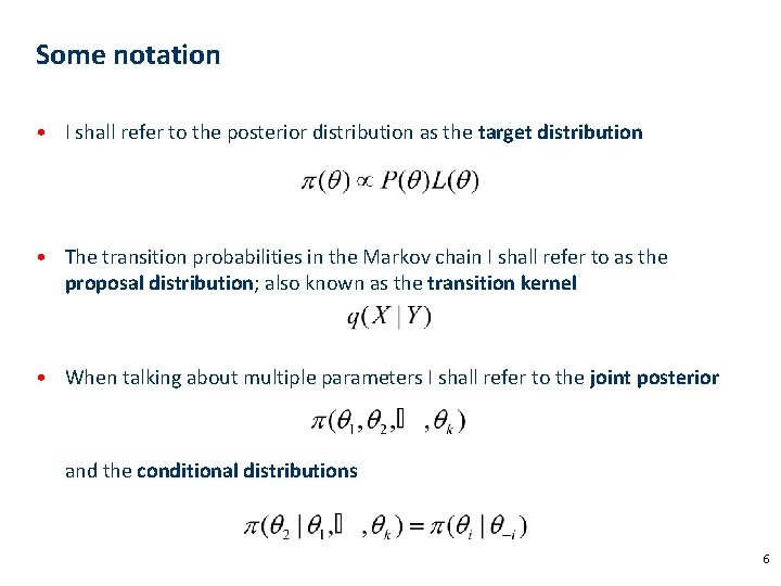
Some notation • I shall refer to the posterior distribution as the target distribution • The transition probabilities in the Markov chain I shall refer to as the proposal distribution; also known as the transition kernel • When talking about multiple parameters I shall refer to the joint posterior and the conditional distributions 6

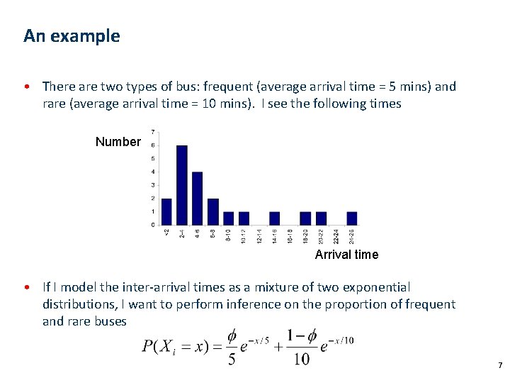
An example • There are two types of bus: frequent (average arrival time = 5 mins) and rare (average arrival time = 10 mins). I see the following times Number Arrival time • If I model the inter-arrival times as a mixture of two exponential distributions, I want to perform inference on the proportion of frequent and rare buses 7

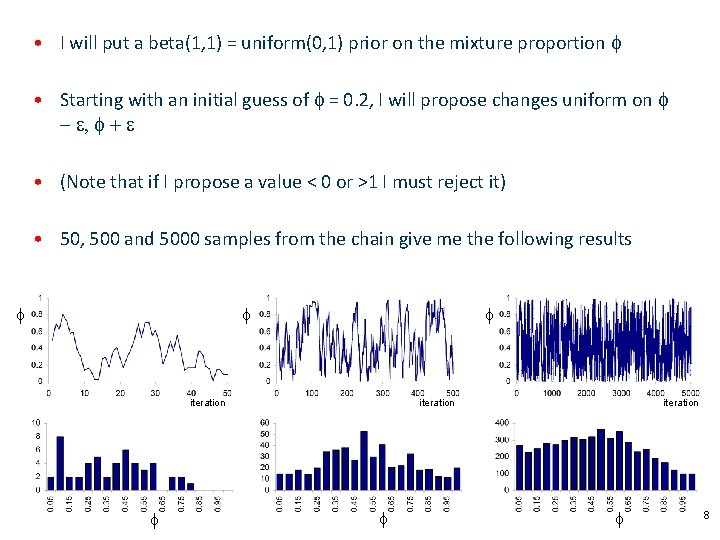
• I will put a beta(1, 1) = uniform(0, 1) prior on the mixture proportion f • Starting with an initial guess of f = 0. 2, I will propose changes uniform on f - e, f + e • (Note that if I propose a value < 0 or >1 I must reject it) • 50, 500 and 5000 samples from the chain give me the following results f f f iteration f 8

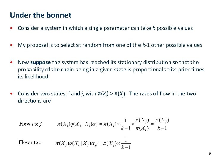
Under the bonnet • Consider a system in which a single parameter can take k possible values • My proposal is to select at random from one of the k-1 other possible values • Now suppose the system has reached its stationary distribution so that the probability of the chain being in a given state is proportional to its prior times its likelihood • Consider two states, i and j, with p(Xi) > p(Xj). The rates of flow in the two directions are Flow i to j Flow j to i 9

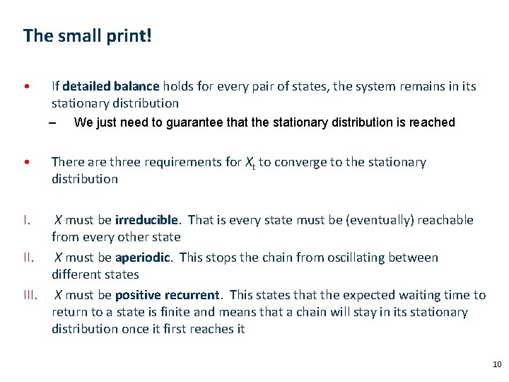
The small print! • If detailed balance holds for every pair of states, the system remains in its stationary distribution – • We just need to guarantee that the stationary distribution is reached There are three requirements for Xt to converge to the stationary distribution I. X must be irreducible. That is every state must be (eventually) reachable from every other state II. X must be aperiodic. This stops the chain from oscillating between different states III. X must be positive recurrent. This states that the expected waiting time to return to a state is finite and means that a chain will stay in its stationary distribution once it first reaches it 10

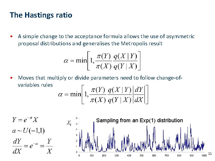
The Hastings ratio • A simple change to the acceptance formula allows the use of asymmetric proposal distributions and generalises the Metropolis result • Moves that multiply or divide parameters need to follow change-ofvariables rules Xt Sampling from an Exp(1) distribution 11

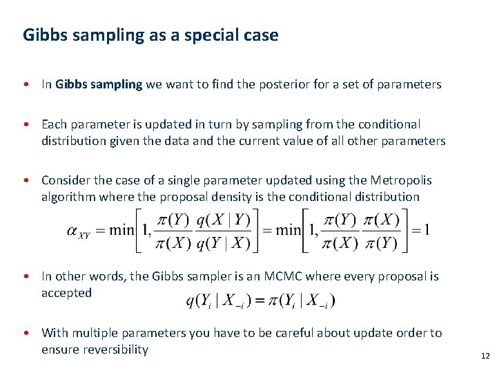
Gibbs sampling as a special case • In Gibbs sampling we want to find the posterior for a set of parameters • Each parameter is updated in turn by sampling from the conditional distribution given the data and the current value of all other parameters • Consider the case of a single parameter updated using the Metropolis algorithm where the proposal density is the conditional distribution • In other words, the Gibbs sampler is an MCMC where every proposal is accepted • With multiple parameters you have to be careful about update order to ensure reversibility 12

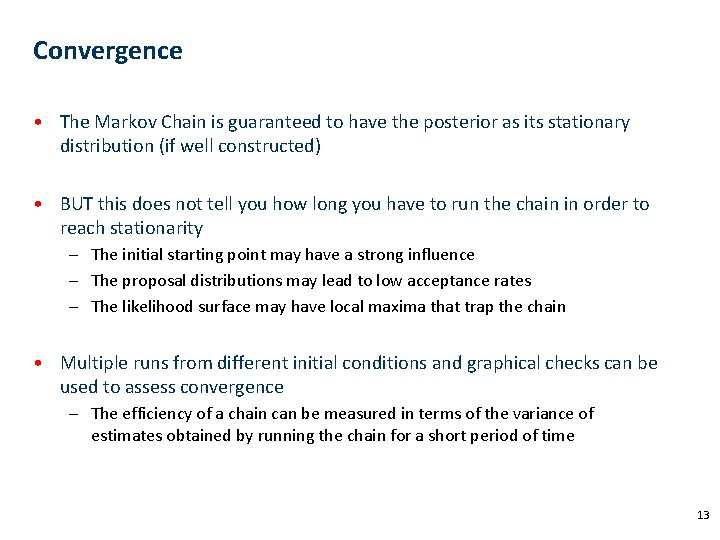
Convergence • The Markov Chain is guaranteed to have the posterior as its stationary distribution (if well constructed) • BUT this does not tell you how long you have to run the chain in order to reach stationarity – The initial starting point may have a strong influence – The proposal distributions may lead to low acceptance rates – The likelihood surface may have local maxima that trap the chain • Multiple runs from different initial conditions and graphical checks can be used to assess convergence – The efficiency of a chain can be measured in terms of the variance of estimates obtained by running the chain for a short period of time 13

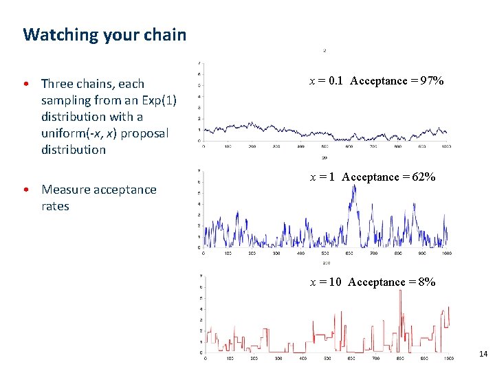
Watching your chain • Three chains, each sampling from an Exp(1) distribution with a uniform(-x, x) proposal distribution • Measure acceptance rates x = 0. 1 Acceptance = 97% x = 1 Acceptance = 62% x = 10 Acceptance = 8% 14

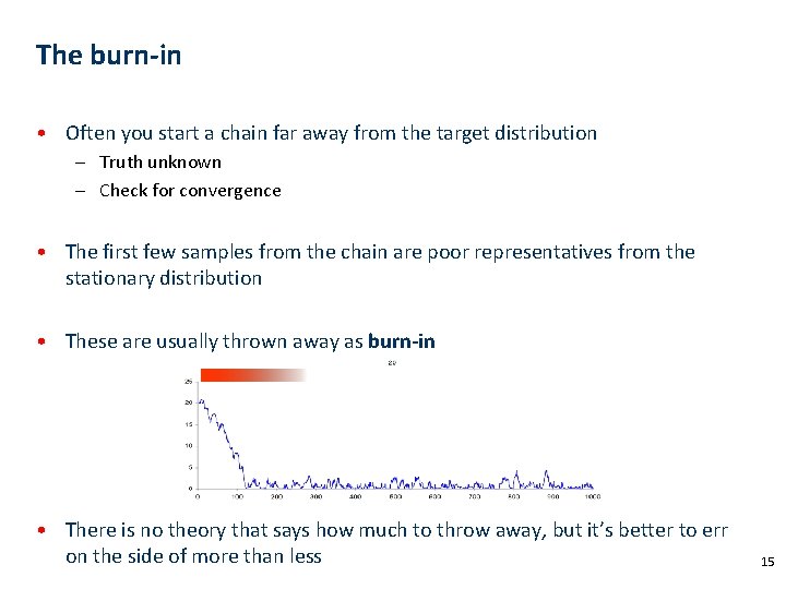
The burn-in • Often you start a chain far away from the target distribution – Truth unknown – Check for convergence • The first few samples from the chain are poor representatives from the stationary distribution • These are usually thrown away as burn-in • There is no theory that says how much to throw away, but it’s better to err on the side of more than less 15

Other uses of MCMC • Looking at marginal effects – Suppose we have a multidimensional parameter, we may just want to know about the marginal posterior distribution of that parameter • Prediction – Given our posterior distribution on parameters, we can predict the distribution of future data by sampling parameters from the posterior and simulating data given those parameters – The posterior predictive distribution is a useful source of goodness-of-fit testing (if predicted data doesn’t look like the data you’ve collected, the model is poor) 16

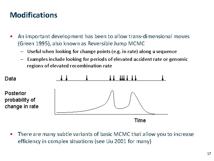
Modifications • An important development has been to allow trans-dimensional moves (Green 1995), also known as Reversible Jump MCMC – Useful when looking for change points (e. g. in rate) along a sequence – Examples include looking for periods of elevated accident rate or genomic regions of elevated recombination rate Data Posterior probability of change in rate Time • There are many subtle variants of basic MCMC that allow you to increase efficiency in complex situations (see Liu 2001 for many) 17

A good read • Markov Chain Monte Carlo in Practice. 1996. eds. Gilks WR, Richardson S and Spiegelhalter DJ. Chapman & Hall/CRC. • Bayesian Data Analysis. 2004. Gelman A, Carlin JB, Stern HS and Rubin DB. Chapman & Hall/CRC. • Monte Carlo Strategies in Scientific Computing. 2001. Liu JS. Springer. Verlag. • Chris Holmes’ short course on Bayesian statistics – http: //www. stats. ox. ac. uk/~cholmes/Courses/BDA/bda_mcmc. pdf 18