Marginal Models and Generalized Estimating Equations 4272021 Xi

Marginal Models and Generalized Estimating Equations 4/27/2021 Xi Chen (Sophia), P. h. D Candidate, MS, MD Department of Biostatistics and Epidemiology Hudson College of Public Health University of Oklahoma Health Sciences Center

Outline • Lecture • Introduction of marginal models and GEE • R demo • In-class exercise 2

Marginal Models • Make inferences about population averages. • The term ‘marginal’ is used here to emphasize that the mean response modelled is conditional only on covariates and not on other responses or random effects. (Remember mixed effects is conditional on random effects) • A feature of marginal models is that the models for the mean and the ‘within-subject association’ (e. g. , covariance) are specified separately. 3

Notation • 4

Features of Marginal Models: • 5

Examples of Marginal Models: Continuous Response • 6

Examples of Marginal Models: Binary Response • 7

Examples of Marginal Models: Count Response • 8

Correlation structure 9

Parameter Estimation for Marginal Models • 10

Introduction of GEE • Generalized estimating equations (GEE) were introduced by Liang and Zeger for handling correlated discrete and continuous outcome variables. • It provides a flexible approach for modelling the mean and the pairwise within-subject association structure. • It can handle inherently unbalanced designs. • It is straightforward to implement. • GEE approach is computationally straightforward. 11

The GEE Estimator • 12

Two-Step Estimation • 13

Properties of GEE estimators • 14

Summary of GEE • GEE is marginal models, which make inferences about population averages. • GEE provides a regression generalized linear models when the responses are correlated/clustered. • It is versatile for modelling the mean and the pairwise within-subject association structure. • GEE model will give valid results with a mispecified correlation structure when the sandwich variance estimator is used 15

R demo • Packages used in R for GEE model • R packages for GEE : geepack, gee, multgee and repolr • geepack contains an ANOVA method that allows us to compare models and perform Wald test. 16

R demo geepack syntax 17

Case Study on Count Data Clinical Trial of Antibiotics for Leprosy • Placebo-controlled clinical trial of 30 patients with leprosy at the Eversley Childs Sanitorium in the Philippines. • Participants were randomized to either of two antibiotics (denoted treatment drug A and B) or to a placebo (denoted treatment drug C). • Baseline data on number of leprosy bacilli at 6 sites of body were recorded. • After several months of treatment, number of bacilli were recorded a second time. • Outcome: Total count of number of leprosy bacilli at 6 sites. • Previously analyzed at follow-up. 18

Mean count of leprosy bacilli at six sites of the body (and variance) at follow-up 19

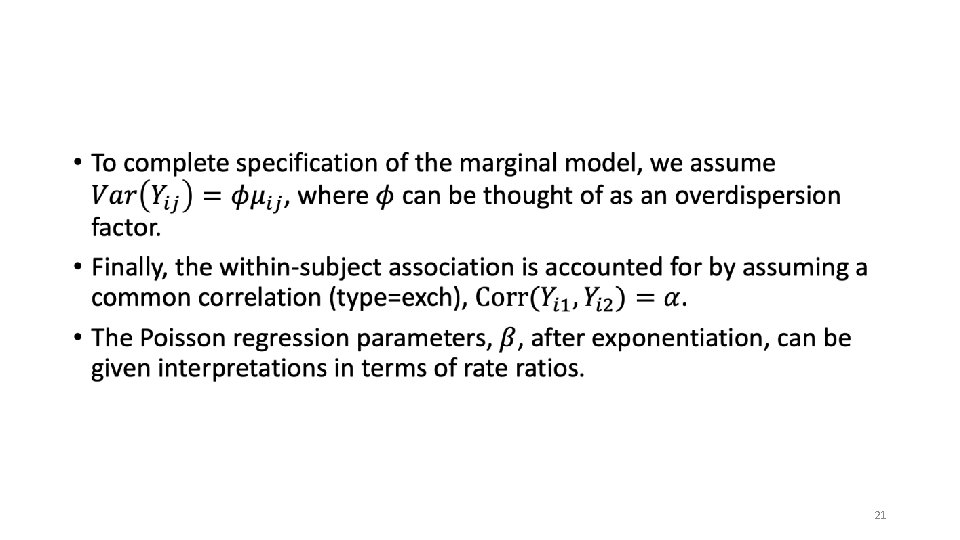
Poisson Regression Model on both baseline and follow-up data • 20

Parameters log-linear regression model 22

Interpretation • 23

R demo • Please see R program 24

Parameter estimates and standard errors from marginal Poisson regression model for the leprosy bacilli data. 25

Interpretation (exp of coefficients) • For placebo group, there is a non-significant reduction in the average number of bacilli of approximately 1%. • The treatment with antibiotic A significantly reduces the average number of bacilli when compared to placebo, with the ratio 0. 57 (95% CI, 0. 4 to 0. 88). There is a significant reduction of approximately 44%. • Estimated pairwise correlation of 0. 74 is relatively large. • Estimated scale parameter of 3. 2 indicates substantial overdispersion. 26

A New Model Combining Drug A and B • 27

Parameter estimates and standard errors from marginal log-linear regression model for the leprosy bacilli data. 28

Interpretation (exp of the coefficients) • The treatment with antibiotics significantly reduces the average number of bacilli when compared to placebo, with the ratio 0. 59 (95% CI, 0. 4 to 0. 87). There is a significant reduction of approximately 40%. • For placebo group, there is a non-significant reduction in the average number of bacilli of approximately 1%. • Estimated pairwise correlation of 0. 74 is relatively large. • Estimated scale parameter of 3. 23 indicates substantial overdispersion. 29