Generalized Estimating Equations GEEs Purpose to introduce GEEs

Generalized Estimating Equations (GEEs) Purpose: to introduce GEEs These are used to model correlated data from • Longitudinal/ repeated measures studies • Clustered/ multilevel studies 1

Outline • Examples of correlated data • Successive generalizations – Normal linear model – Generalized linear model – GEE • Estimation • Example: stroke data – exploratory analysis – modelling 2

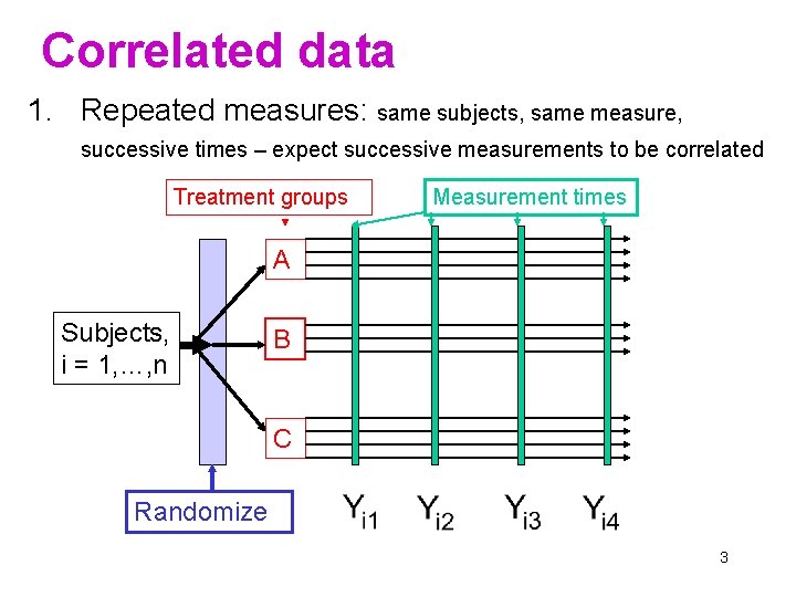
Correlated data 1. Repeated measures: same subjects, same measure, successive times – expect successive measurements to be correlated Treatment groups Measurement times A Subjects, i = 1, …, n B C Randomize 3

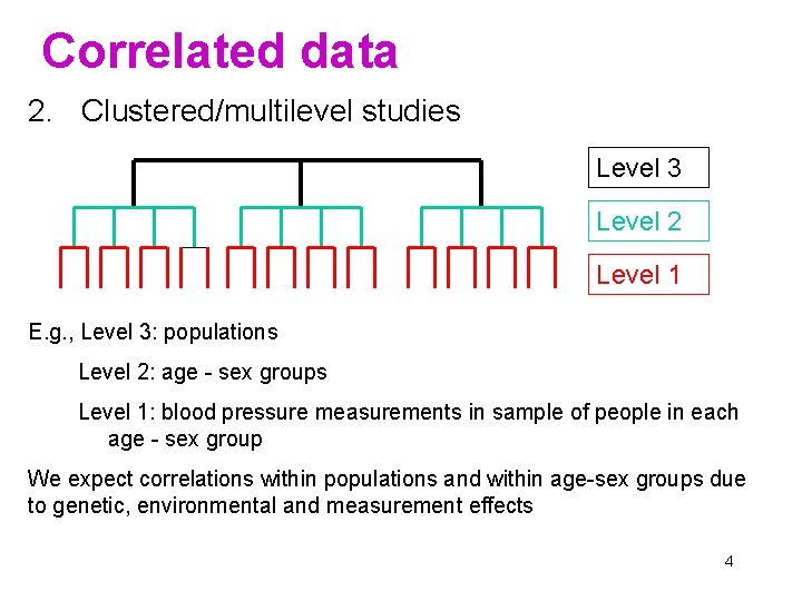
Correlated data 2. Clustered/multilevel studies Level 3 Level 2 Level 1 E. g. , Level 3: populations Level 2: age - sex groups Level 1: blood pressure measurements in sample of people in each age - sex group We expect correlations within populations and within age-sex groups due to genetic, environmental and measurement effects 4

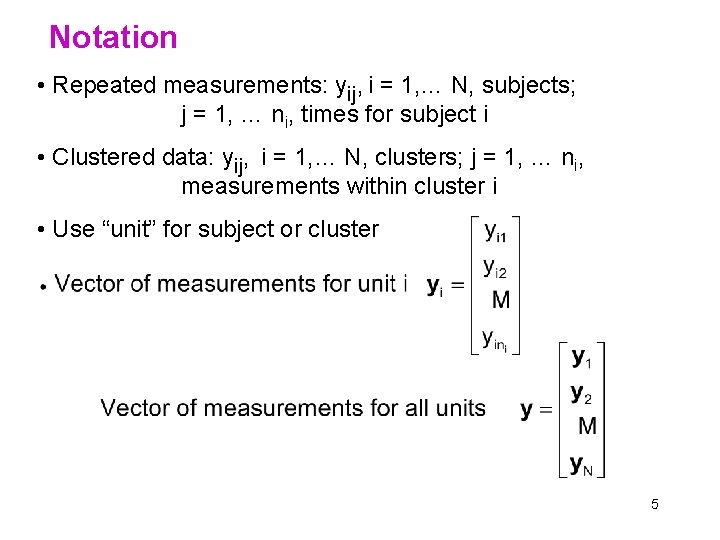
Notation • Repeated measurements: yij, i = 1, … N, subjects; j = 1, … ni, times for subject i • Clustered data: yij, i = 1, … N, clusters; j = 1, … ni, measurements within cluster i • Use “unit” for subject or cluster 5

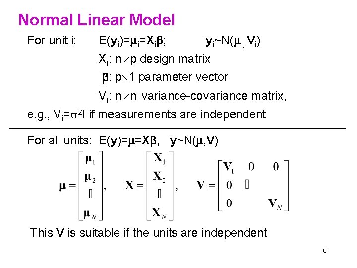
Normal Linear Model For unit i: E(yi)= i=Xi ; yi~N( i, Vi) Xi: ni p design matrix : p 1 parameter vector Vi: ni ni variance-covariance matrix, e. g. , Vi= 2 I if measurements are independent For all units: E(y)= =X , y~N( , V) This V is suitable if the units are independent 6

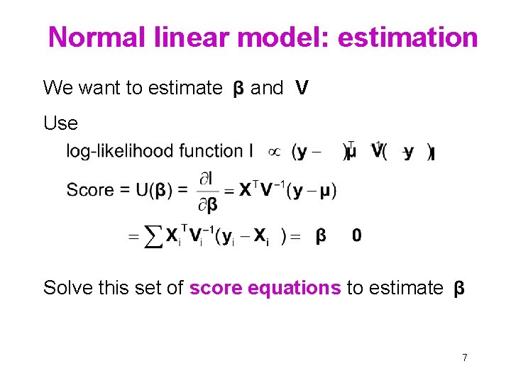
Normal linear model: estimation We want to estimate and V Use Solve this set of score equations to estimate 7

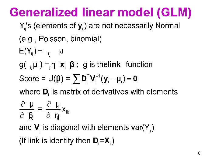
Generalized linear model (GLM) 8

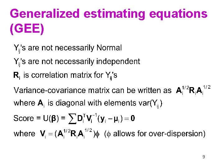
Generalized estimating equations (GEE) 9

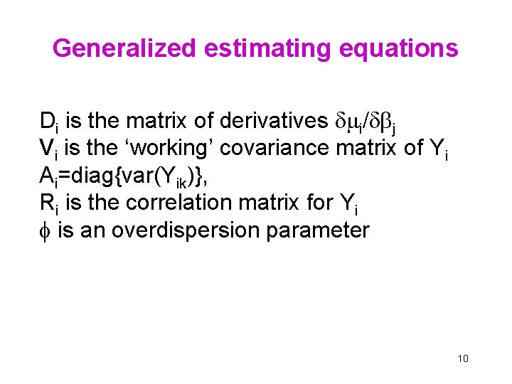
Generalized estimating equations Di is the matrix of derivatives i/ j Vi is the ‘working’ covariance matrix of Yi Ai=diag{var(Yik)}, Ri is the correlation matrix for Yi is an overdispersion parameter 10

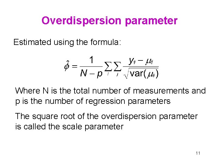
Overdispersion parameter Estimated using the formula: Where N is the total number of measurements and p is the number of regression parameters The square root of the overdispersion parameter is called the scale parameter 11

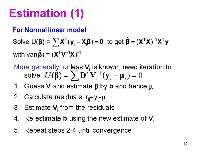
Estimation (1) More generally, unless Vi is known, need iteration to solve 1. Guess Vi and estimate by b and hence 2. Calculate residuals, rij=yij- ij 3. Estimate Vi from the residuals 4. Re-estimate b using the new estimate of Vi 5. Repeat steps 2 -4 until convergence 12

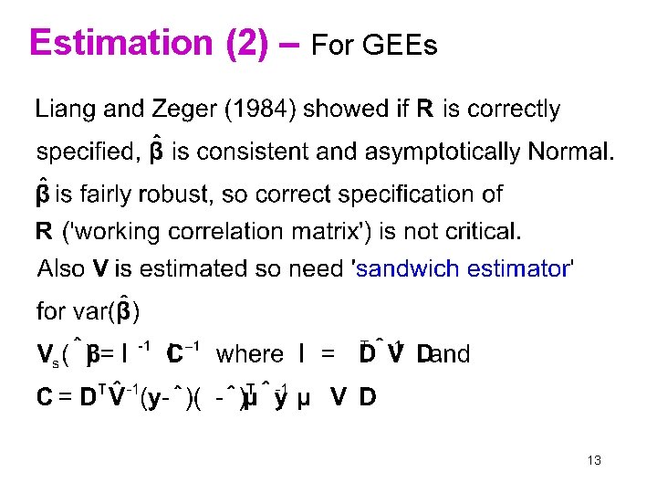
Estimation (2) – For GEEs 13

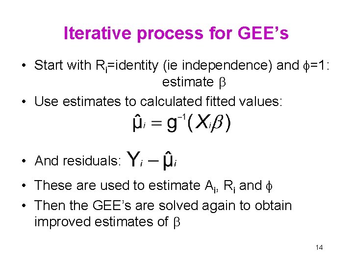
Iterative process for GEE’s • Start with Ri=identity (ie independence) and =1: estimate • Use estimates to calculated fitted values: • And residuals: • These are used to estimate Ai, Ri and • Then the GEE’s are solved again to obtain improved estimates of 14

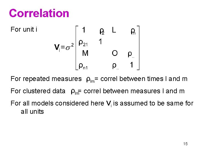
Correlation For unit i For repeated measures For clustered data = correl between times l and m = correl between measures l and m For all models considered here Vi is assumed to be same for all units 15

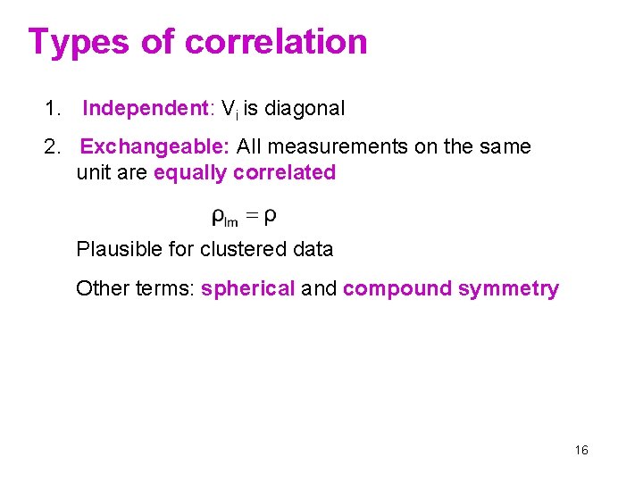
Types of correlation 1. Independent: Vi is diagonal 2. Exchangeable: All measurements on the same unit are equally correlated Plausible for clustered data Other terms: spherical and compound symmetry 16

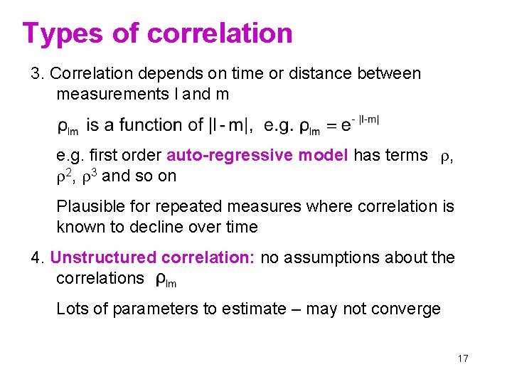
Types of correlation 3. Correlation depends on time or distance between measurements l and m e. g. first order auto-regressive model has terms , 2, 3 and so on Plausible for repeated measures where correlation is known to decline over time 4. Unstructured correlation: no assumptions about the correlations Lots of parameters to estimate – may not converge 17

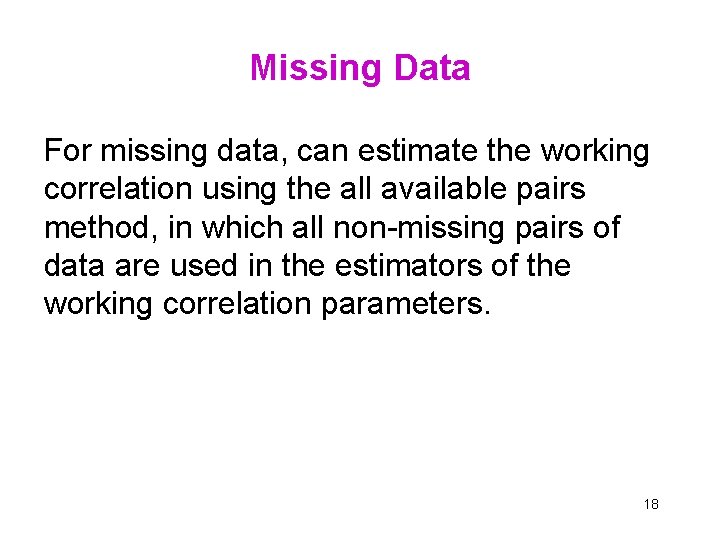
Missing Data For missing data, can estimate the working correlation using the all available pairs method, in which all non-missing pairs of data are used in the estimators of the working correlation parameters. 18

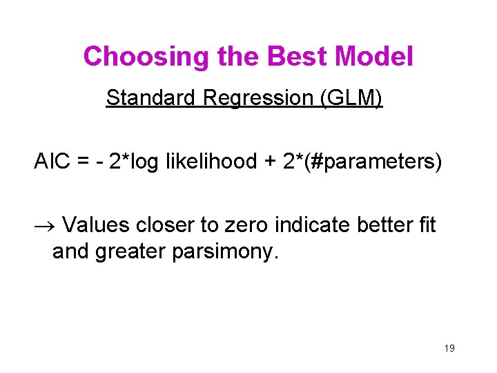
Choosing the Best Model Standard Regression (GLM) AIC = - 2*log likelihood + 2*(#parameters) ® Values closer to zero indicate better fit and greater parsimony. 19

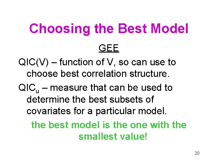
Choosing the Best Model GEE QIC(V) – function of V, so can use to choose best correlation structure. QICu – measure that can be used to determine the best subsets of covariates for a particular model. the best model is the one with the smallest value! 20

Other approaches – alternatives to GEEs 1. Multivariate modelling – treat all measurements on same unit as dependent variables (even though they are measurements of the same variable) and model them simultaneously (Hand Crowder, 1996) e. g. , SPSS uses this approach (with exchangeable correlation) for repeated measures ANOVA 21

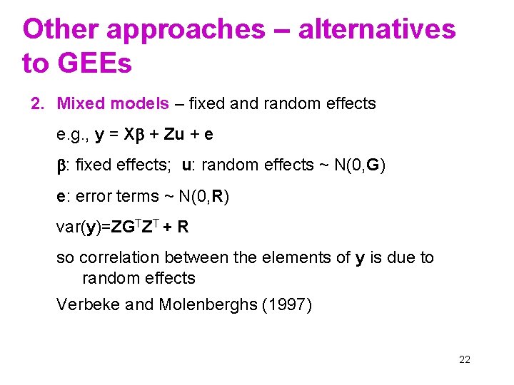
Other approaches – alternatives to GEEs 2. Mixed models – fixed and random effects e. g. , y = X + Zu + e : fixed effects; u: random effects ~ N(0, G) e: error terms ~ N(0, R) var(y)=ZGTZT + R so correlation between the elements of y is due to random effects Verbeke and Molenberghs (1997) 22

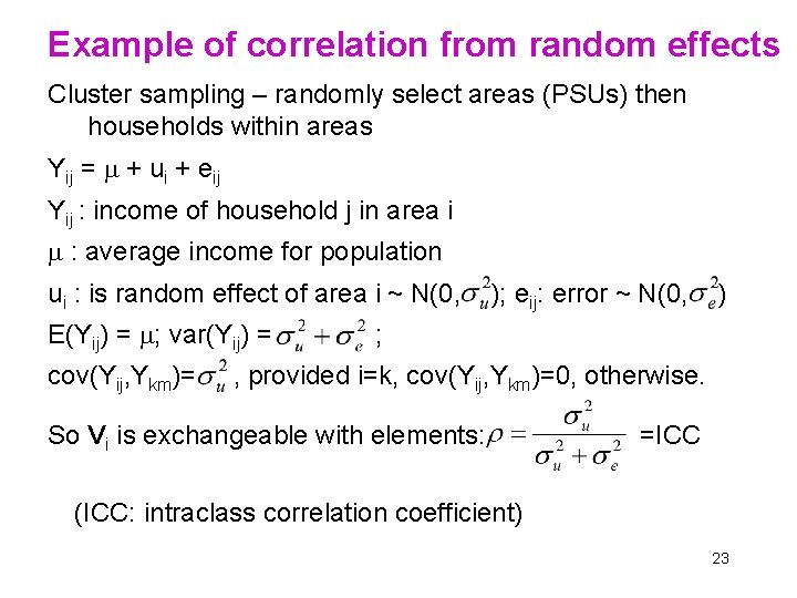
Example of correlation from random effects Cluster sampling – randomly select areas (PSUs) then households within areas Yij = + ui + eij Yij : income of household j in area i : average income for population ui : is random effect of area i ~ N(0, E(Yij) = ; var(Yij) = cov(Yij, Ykm)= ); eij: error ~ N(0, ) ; , provided i=k, cov(Yij, Ykm)=0, otherwise. So Vi is exchangeable with elements: =ICC (ICC: intraclass correlation coefficient) 23

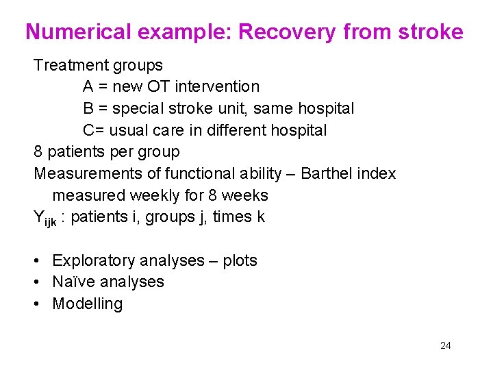
Numerical example: Recovery from stroke Treatment groups A = new OT intervention B = special stroke unit, same hospital C= usual care in different hospital 8 patients per group Measurements of functional ability – Barthel index measured weekly for 8 weeks Yijk : patients i, groups j, times k • Exploratory analyses – plots • Naïve analyses • Modelling 24

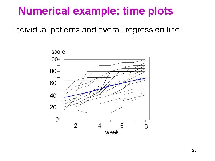
Numerical example: time plots Individual patients and overall regression line 25

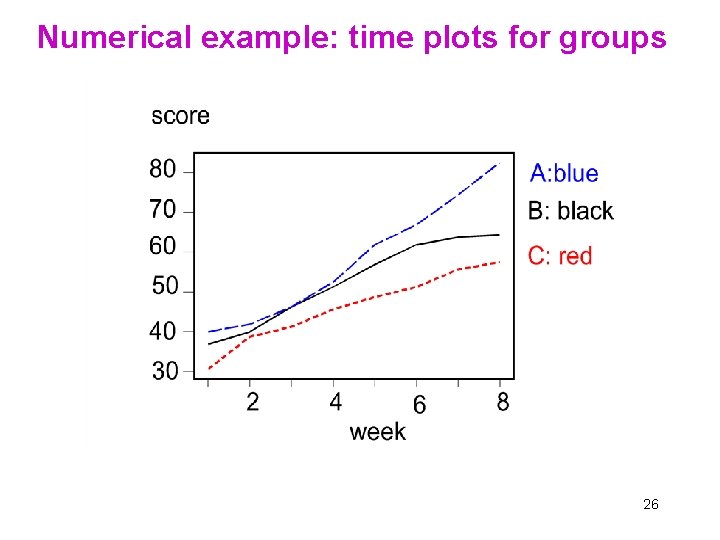
Numerical example: time plots for groups 26

Numerical example: research questions • Primary question: do slopes differ (i. e. do treatments have different effects)? • Secondary question: do intercepts differ (i. e. are groups same initially)? 27

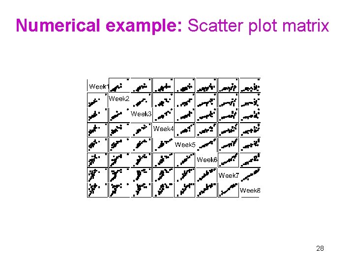
Numerical example: Scatter plot matrix 28

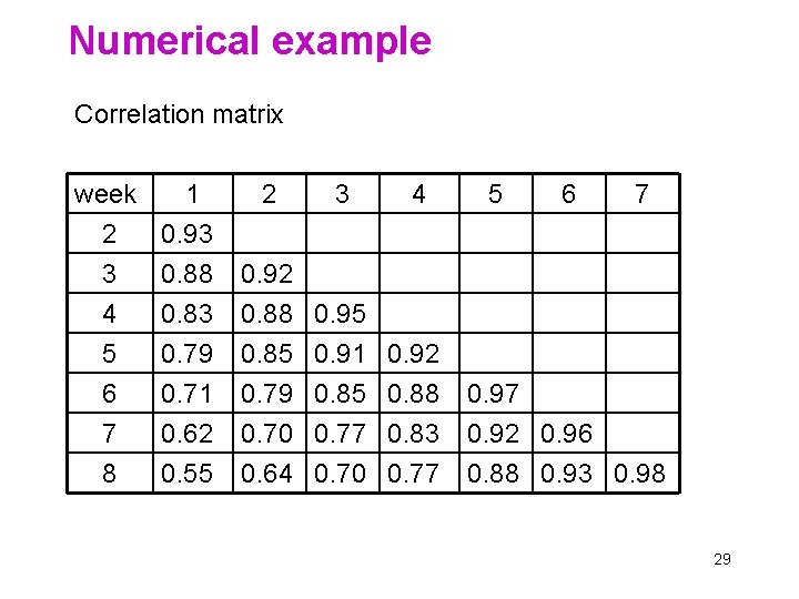
Numerical example Correlation matrix week 1 2 0. 93 3 0. 88 4 0. 83 5 6 7 8 0. 79 0. 71 0. 62 0. 55 2 3 4 5 6 7 0. 92 0. 88 0. 95 0. 85 0. 79 0. 70 0. 64 0. 91 0. 85 0. 77 0. 70 0. 92 0. 88 0. 83 0. 77 0. 92 0. 96 0. 88 0. 93 0. 98 29

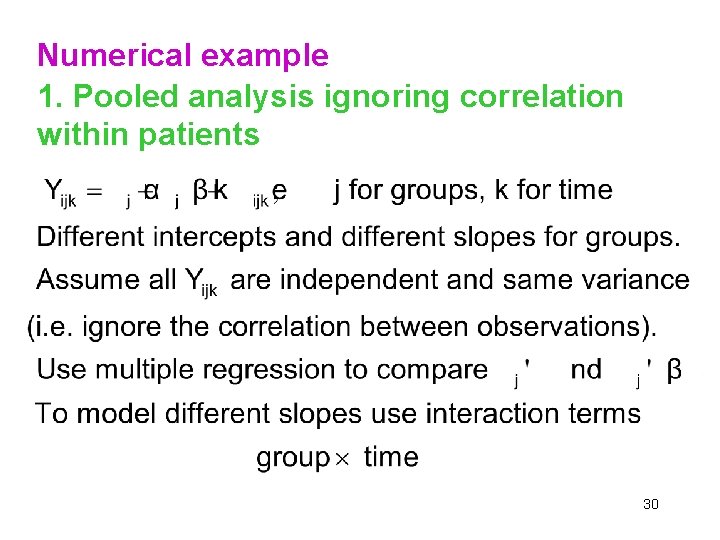
Numerical example 1. Pooled analysis ignoring correlation within patients 30

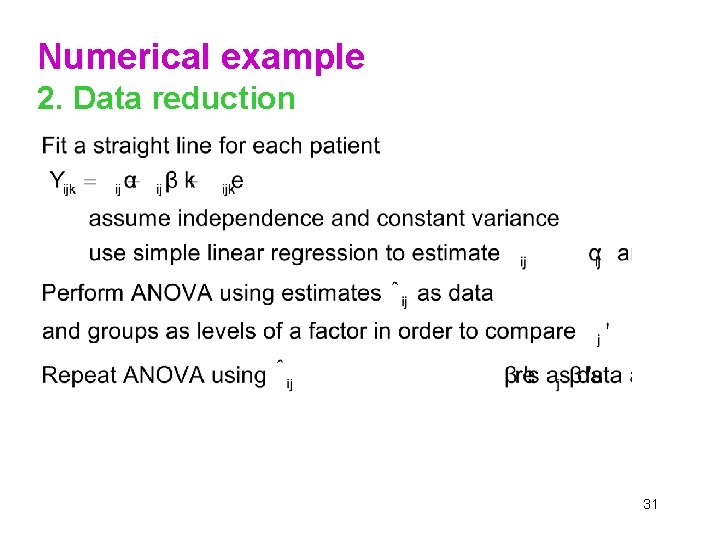
Numerical example 2. Data reduction 31

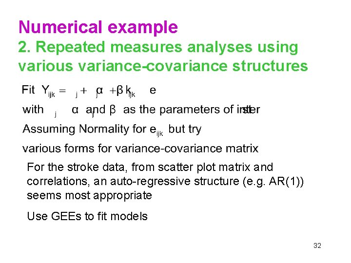
Numerical example 2. Repeated measures analyses using various variance-covariance structures For the stroke data, from scatter plot matrix and correlations, an auto-regressive structure (e. g. AR(1)) seems most appropriate Use GEEs to fit models 32

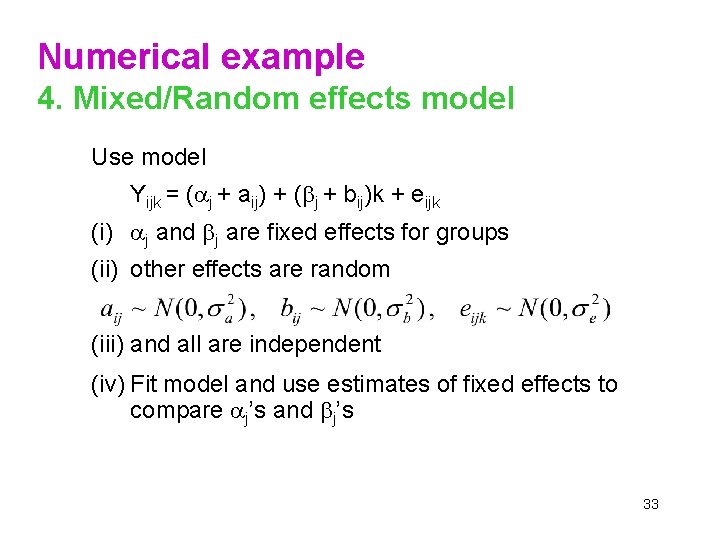
Numerical example 4. Mixed/Random effects model Use model Yijk = ( j + aij) + ( j + bij)k + eijk (i) j and j are fixed effects for groups (ii) other effects are random (iii) and all are independent (iv) Fit model and use estimates of fixed effects to compare j’s and j’s 33

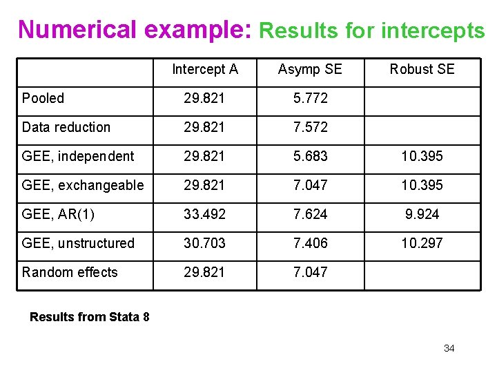
Numerical example: Results for intercepts Intercept A Asymp SE Robust SE Pooled 29. 821 5. 772 Data reduction 29. 821 7. 572 GEE, independent 29. 821 5. 683 10. 395 GEE, exchangeable 29. 821 7. 047 10. 395 GEE, AR(1) 33. 492 7. 624 9. 924 GEE, unstructured 30. 703 7. 406 10. 297 Random effects 29. 821 7. 047 Results from Stata 8 34

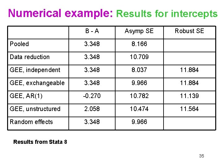
Numerical example: Results for intercepts B-A Asymp SE Robust SE Pooled 3. 348 8. 166 Data reduction 3. 348 10. 709 GEE, independent 3. 348 8. 037 11. 884 GEE, exchangeable 3. 348 9. 966 11. 884 GEE, AR(1) -0. 270 10. 782 11. 139 GEE, unstructured 2. 058 10. 474 11. 564 Random effects 3. 348 9. 966 Results from Stata 8 35

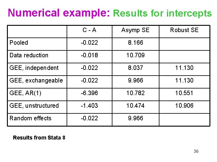
Numerical example: Results for intercepts C-A Asymp SE Robust SE Pooled -0. 022 8. 166 Data reduction -0. 018 10. 709 GEE, independent -0. 022 8. 037 11. 130 GEE, exchangeable -0. 022 9. 966 11. 130 GEE, AR(1) -6. 396 10. 782 10. 551 GEE, unstructured -1. 403 10. 474 10. 906 Random effects -0. 022 9. 966 Results from Stata 8 36

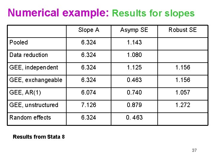
Numerical example: Results for slopes Slope A Asymp SE Robust SE Pooled 6. 324 1. 143 Data reduction 6. 324 1. 080 GEE, independent 6. 324 1. 125 1. 156 GEE, exchangeable 6. 324 0. 463 1. 156 GEE, AR(1) 6. 074 0. 740 1. 057 GEE, unstructured 7. 126 0. 879 1. 272 Random effects 6. 324 0. 463 Results from Stata 8 37

Numerical example: Results for slopes B-A Asymp SE Robust SE Pooled -1. 994 1. 617 Data reduction -1. 994 1. 528 GEE, independent -1. 994 1. 592 1. 509 GEE, exchangeable -1. 994 0. 655 1. 509 GEE, AR(1) -2. 142 1. 047 1. 360 GEE, unstructured -3. 556 1. 243 1. 563 Random effects -1. 994 0. 655 Results from Stata 8 38

Numerical example: Results for slopes C-A Asymp SE Robust SE Pooled -2. 686 1. 617 Data reduction -2. 686 1. 528 GEE, independent -2. 686 1. 592 1. 502 GEE, exchangeable -2. 686 0. 655 1. 509 GEE, AR(1) -2. 236 1. 047 1. 504 GEE, unstructured -4. 012 1. 243 1. 598 Random effects -2. 686 0. 655 Results from Stata 8 39

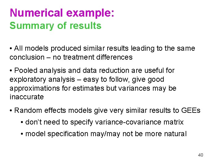
Numerical example: Summary of results • All models produced similar results leading to the same conclusion – no treatment differences • Pooled analysis and data reduction are useful for exploratory analysis – easy to follow, give good approximations for estimates but variances may be inaccurate • Random effects models give very similar results to GEEs • don’t need to specify variance-covariance matrix • model specification may/may not be more natural 40