MA 354 Computer Assisted Math Modeling Math Modeling

MA 354 Computer Assisted Math Modeling: Math Modeling Introduction

Outline A. Three Course Objectives 1. Model literacy: understanding a typical model description 2. Model Analysis: understanding the information a model provides (and its relevance to the real world. . ) 3. Building Models: choose assumptions, write description using mathematical notation, build the model in software B. What is a “model”? Model= description of relationships among quantities. C. Building a Model D. Model Classifications

A. Course Objectives

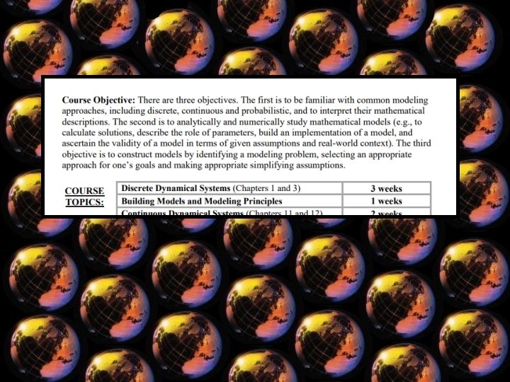
Course Objectives • Objective 1: Model Literacy The first objective is the ability to “read” models and understand what the important features being communicated from a given mathematical description.

Interpreting the Mathematical Description of a Model Implicit and discrete: System of equations: Exotic or unfamiliar model: (statistical mechanics)

Course Objectives • Objective 2: Model Analysis and Validity The second objective is to study mathematical models analytically and numerically. The mathematical conclusions thus drawn are interpreted in terms of the real-world problem that was modeled, thereby ascertaining the validity of the model.

Course Objectives • Objective 3: Model Construction The third objective is to learn to build models of real-world phenomena by making appropriate simplifying assumptions and identifying key factors.

MA 354 Computer Assisted Math Modeling: Math Modeling Introduction

Outline A. Three Course Objectives 1. Model literacy: understanding a typical model description 2. Model Analysis: understanding the information a model provides (and its relevance to the real world. . ) 3. Building Models: choose assumptions, write description using mathematical notation, build the model in software B. What is a “model”? Model= description of relationships among quantities. C. Building a Model D. Model Classifications

B. What is a model?

Not the type of model we mean:

Not the type of model we mean:

Not the type of model we mean:

For us, a model is: • A set of variables {u, v, w, …} – Selected based on those the a phenomenon of interest is hypothesized to depend on – Together define a system • A description of the functional quantitative relationship of those variables

Simple example: •

“Interesting” examples: •

“Interesting” examples: •

Classic Modeling Examples

Classic Modeling Examples Malthusian Population Growth (exponential)

Classic Modeling Examples Logistic Population Growth

Classic Modeling Examples Malthusian Population Growth (exponential)

Classic Modeling Examples Malthusian Population Growth (exponential)

Classic Modeling Examples Logistic Population Growth

Classic Modeling Examples Epidemic Spread: Kermack-Mc. Kendrick 1927 SIR Model

Classic Modeling Examples Epidemic Spread: Kermack-Mc. Kendrick 1927 SIR Model Short time periods: exponential increase in cases

Classic Modeling Examples Epidemic Spread: Kermack-Mc. Kendrick 1927 SIR Model Long term behavior: more complex

C. Building Models

Model Construction. . • A modeler must first select a number of variables, and then determine and describe their relationship. • Note: pragmatically, simplicity and computational efficiency often trump accuracy. (A mathematical model describes a system with variables {u, v, w, …} by describing the functional relationship of those variables. )

Model Construction. . • A modeler must first select a number of variables, and then determine and describe their relationship. • Note: pragmatically, simplicity and computational efficiency often trump accuracy. (A mathematical model describes a system with variables {u, v, w, …} by describing the functional relationship of those variables. )

Model Construction. . • A modeler must first select a number of variables, and then determine and describe their relationship. • Note: pragmatically, simplicity and computational efficiency often trump accuracy. The value of a model is in its ability to make an accurate or (A mathematical model describes a system with variables useful set of predictions, not in all possible aspects. of {u, v, w, …} by describing the realism functional relationship variables. ) those

Principles of Model Design • Model design: – Models are extreme simplifications! – A model should be designed to address a particular question; for a focused application. – The model should focus on the smallest subset of attributes to answer the question. – This is a feature, not a problem. • Model validation: – Does the model reproduce relevant behavior? Necessary but not sufficient. – New predictions are empirically confirmed. Better • Model value: – Better understanding of known phenomena – does the model allow investigation of a question of interest? – New phenomena predicted that motivate further experiments.

Classifying Models

In Class Assignment (submit on Sakai / optional) • • Choose a topic Find a mathematical model on that topic Share the mathematical model you found with a screen shot and/or a link. Write a brief(!) description of the model. (What does it do and what sort of model is it? )

Classifying Models • By application (ecological, epidemiological, etc) • Discrete or continuous? • Stochastic or deterministic? • Simple or Sophisticated • Validated, Hypothetical or Invalidated

DISCRETE OR CONTINUOUS?

Discrete verses Continuous • Discrete: – Values are separate and distinct (definition) – Either limited range of values (e. g. , measurements taken to nearest quarter inch) – Or measurements taken at discrete time points (e. g. , every year or once a day, etc. ) • Continuous – Values taken from the continuum (real line) – Instantaneous, continuous measurement (in theory)

Modeling Approaches Continuous Verses Discrete • Continuous Approaches (differential equations) • Discrete Approaches (lattices)

Modeling Approaches Continuous Verses Discrete • Continuous Approaches (smooth equations) • Discrete Approaches (discrete representation)

Continuous Models • Good models for HUGE populations (1023), where “average” behavior is an appropriate description. • Usually: ODEs, PDEs • Typically describe “fields” and long-range effects • Large-scale events – Diffusion: Fick’s Law – Fluids: Navier-Stokes Equation

Continuous Models http: //math. uc. edu/~srdjan/movie 2. gif Biological applications: Cells/Molecules = density field. Rotating Vortices http: //www. eng. vt. edu/fluids/msc/gallery/gall. htm

Discrete Models • E. g. , cellular automata. • Typically describe micro-scale events and short-range interactions • “Local rules” define particle behavior • Space is discrete => space is a grid. • Time is discrete => “simulations” and “timesteps” • Good models when a small number of elements can have a large, stochastic effect on entire system.

Hybrid Models • Mix of discrete and continuous components • Very powerful, custom-fit for each application • Example: Modeling Tumor Growth – Discrete model of the biological cells – Continuum model for diffusion of nutrients and oxygen – Yi Jiang and colleagues:

Modeling Approaches Deterministic Verses Stochastic • Deterministic Approaches – Solution is always the same and represents the average behavior of a system. • Stochastic Approaches – A random number generator is used. – Solution is a little different every time you run a simulation. • Examples: Compare particle diffusion, hurricane paths.

Stochastic Models • Accounts for random, probabilistic phenomena by considering specific possibilities. • In practice, the generation of random numbers is required. • Different result each time.

Deterministic Models • One result. • Thus, analytic results possible. • In a process with a probabilistic component, represents average result.

Stochastic vs Deterministic • Averaging over possibilities deterministic • Considering specific possibilities stochastic • Example: Random Motion of a Particle – Deterministic: The particle position is given by a field describing the set of likely positions. – Stochastic: A particular path if generated.

Other Ways that Model Differ • What is being described? • What question is the model trying to investigate? • Example: An epidemiology model that describes the spread of a disease throughout a region, verses one that tries to describe the course of a disease in one patient.

Increasing the Number of Variables Increases the Complexity • What are the variables? – A simple model for tumor growth depends upon time. – A less simple model for tumor growth depends upon time and average oxygen levels. – A complex model for tumor growth depends upon time and oxygen levels that vary over space.

Spatially Explicit Models • • • Spatial variables (x, y) or (r, ) Generally, much more sophisticated. Generally, much more complex! ODE: no spatial variables PDE: spatial variables

In Class Assignment (submit on Sakai / optional) • • Choose a topic Find a mathematical model on that topic Share the mathematical model you found with a screen shot and/or a link. Write a brief(!) description of the model. (What does it do and what sort of model is it? )