Lowx physics at HERA A M CooperSarkar Copenhagen

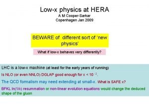
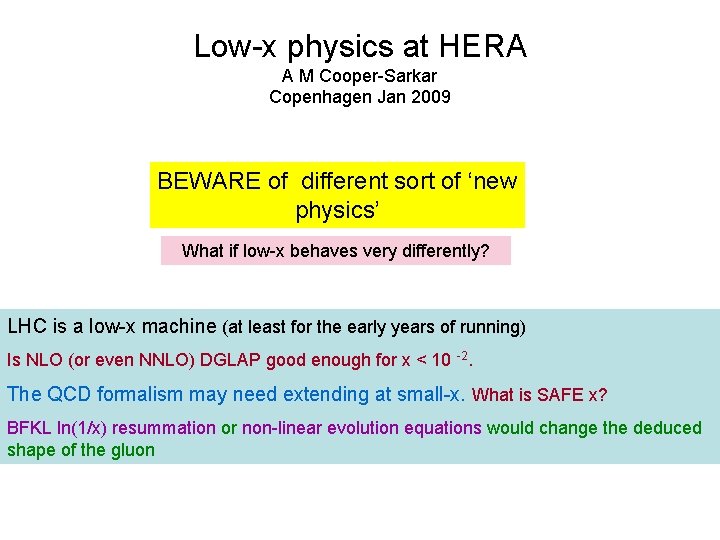
Low-x physics at HERA A M Cooper-Sarkar Copenhagen Jan 2009 BEWARE of different sort of ‘new physics’ What if low-x behaves very differently? LHC is a low-x machine (at least for the early years of running) Is NLO (or even NNLO) DGLAP good enough for x < 10 -2. The QCD formalism may need extending at small-x. What is SAFE x? BFKL ln(1/x) resummation or non-linear evolution equations would change the deduced shape of the gluon

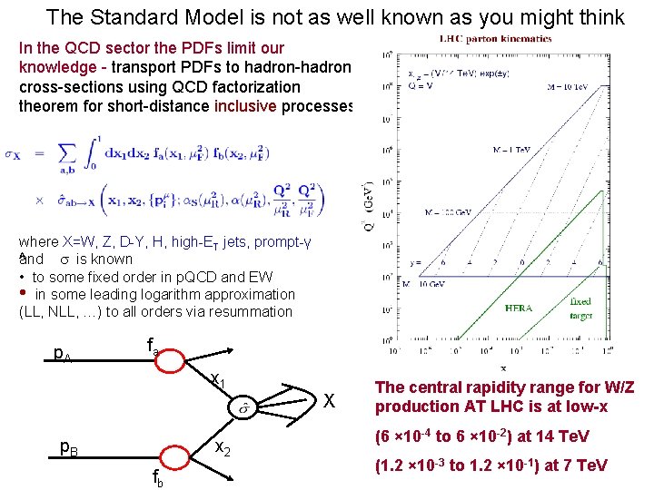
The Standard Model is not as well known as you might think In the QCD sector the PDFs limit our knowledge - transport PDFs to hadron-hadron cross-sections using QCD factorization theorem for short-distance inclusive processes where X=W, Z, D-Y, H, high-ET jets, prompt-γ ^ and is known • to some fixed order in p. QCD and EW • in some leading logarithm approximation (LL, NLL, …) to all orders via resummation p. A fa x 1 X p. B x 2 fb The central rapidity range for W/Z production AT LHC is at low-x (6 × 10 -4 to 6 × 10 -2) at 14 Te. V (1. 2 × 10 -3 to 1. 2 × 10 -1) at 7 Te. V

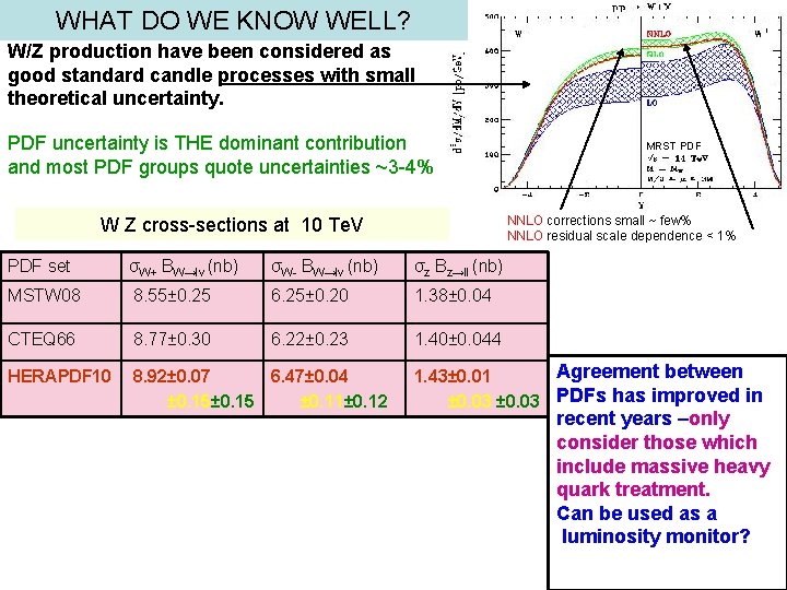
WHAT DO WE KNOW WELL? W/Z production have been considered as good standard candle processes with small theoretical uncertainty. PDF uncertainty is THE dominant contribution and most PDF groups quote uncertainties ~3 -4% MRST PDF NNLO corrections small ~ few% NNLO residual scale dependence < 1% W Z cross-sections at 10 Te. V PDF set σW+ BW→lν (nb) σW- BW→lν (nb) σz Bz→ll (nb) MSTW 08 8. 55± 0. 25 6. 25± 0. 20 1. 38± 0. 04 CTEQ 66 8. 77± 0. 30 6. 22± 0. 23 1. 40± 0. 044 HERAPDF 10 8. 92± 0. 07 6. 47± 0. 04 ± 0. 15 ± 0. 11± 0. 12 Agreement between 1. 43± 0. 01 ± 0. 03 PDFs has improved in recent years –only consider those which include massive heavy quark treatment. Can be used as a luminosity monitor?

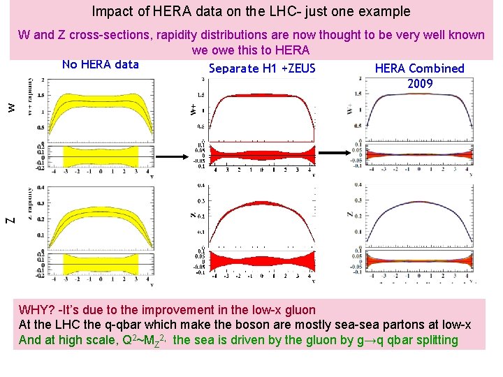
Impact of HERA data on the LHC- just one example Z w W and Z cross-sections, rapidity distributions are now thought to be very well known we owe this to HERA No HERA data Separate H 1 +ZEUS HERA Combined 2009 WHY? -It’s due to the improvement in the low-x gluon At the LHC the q-qbar which make the boson are mostly sea-sea partons at low-x And at high scale, Q 2~MZ 2, the sea is driven by the gluon by g→q qbar splitting

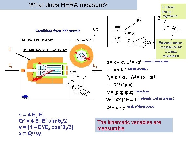
What does HERA measure? Leptonic tensor calculable 2 Lμν Wμν dσ ~ Hadronic tensorconstrained by Lorentz invariance E Ee Ep q = k – k’, Q 2 = -q 2 s= (p + k)2 momentum transfer c. of m. energy 2 Px = p + q , W 2 = (p + q)2 x = Q 2 / (2 p. q) y = (p. q)/(p. k) inelasticity W 2 = Q 2 (1/x – 1) hadronic c. of m energy 2 Q 2 = s x y s = 4 Ee Ep Q 2 = 4 Ee E’ sin 2θe/2 y = (1 – E’/Ee cos 2θe/2) x = Q 2/sy scale of the process The kinematic variables are measurable

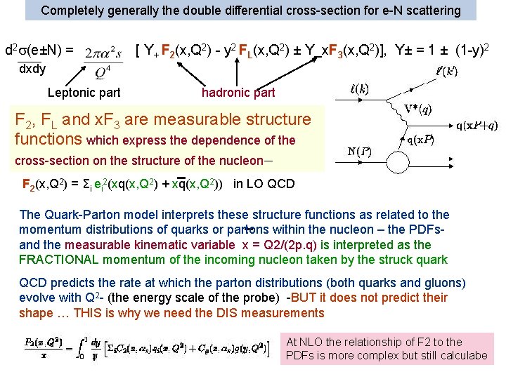
Completely generally the double differential cross-section for e-N scattering d 2 (e±N) = [ Y+ F 2(x, Q 2) - y 2 FL(x, Q 2) ± Y_x. F 3(x, Q 2)], Y± = 1 ± (1 -y)2 dxdy Leptonic part hadronic part F 2, FL and x. F 3 are measurable structure functions which express the dependence of the cross-section on the structure of the nucleon– F 2(x, Q 2) = Σi ei 2(xq(x, Q 2) + xq(x, Q 2)) in LO QCD The Quark-Parton model interprets these structure functions as related to the momentum distributions of quarks or partons within the nucleon – the PDFsand the measurable kinematic variable x = Q 2/(2 p. q) is interpreted as the FRACTIONAL momentum of the incoming nucleon taken by the struck quark QCD predicts the rate at which the parton distributions (both quarks and gluons) evolve with Q 2 - (the energy scale of the probe) -BUT it does not predict their shape … THIS is why we need the DIS measurements At NLO the relationship of F 2 to the PDFs is more complex but still calculabe

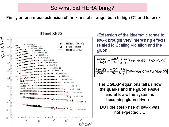
So what did HERA bring? Firstly an enormous extension of the kinematic range: both to high Q 2 and to low-x. • Extension of the kinematic range to low-x brought very interesting effects related to Scaling Violation and the gluon. The DGLAP equations tell us how the quarks and the gluon evolve and at low-x the system is becoming gluon driven… BUT the steep rise at low-x was not expected…. .

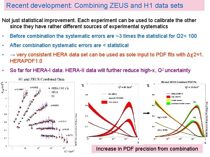
Recent development: Combining ZEUS and H 1 data sets Not just statistical improvement. Each experiment can be used to calibrate the other since they have rather different sources of experimental systematics • Before combination the systematic errors are ~3 times the statistical for Q 2< 100 • After combination systematic errors are < statistical • → very consistent HERA data set can be used as sole input to PDF fits with Δχ2=1. HERAPDF 1. 0 • So far for HERA-I data. HERA-II data will further reduce high-x, Q 2 uncertainty Increase in PDF precision from combination

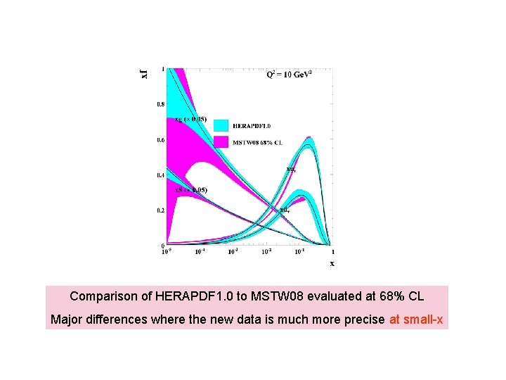
Comparison of HERAPDF 1. 0 to MSTW 08 evaluated at 68% CL Major differences where the new data is much more precise at small-x

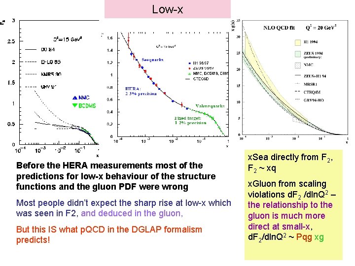
Low-x Before the HERA measurements most of the predictions for low-x behaviour of the structure functions and the gluon PDF were wrong Most people didn’t expect the sharp rise at low-x which was seen in F 2, and deduced in the gluon, But this IS what p. QCD in the DGLAP formalism predicts! x. Sea directly from F 2, F 2 ~ xq x. Gluon from scaling violations d. F 2 /dln. Q 2 – the relationship to the gluon is much more direct at small-x, d. F 2/dln. Q 2 ~ Pqg xg

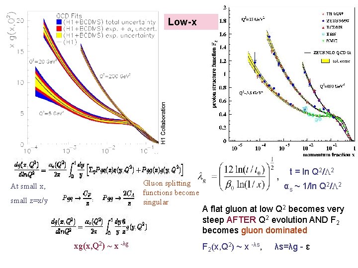
Low-x t = ln Q 2/ 2 Gluon splitting functions become singular At small x, small z=x/y xg(x, Q 2) ~ x -λg αs ~ 1/ln Q 2/ 2 A flat gluon at low Q 2 becomes very steep AFTER Q 2 evolution AND F 2 becomes gluon dominated F 2(x, Q 2) ~ x -λs, λs=λg - ε

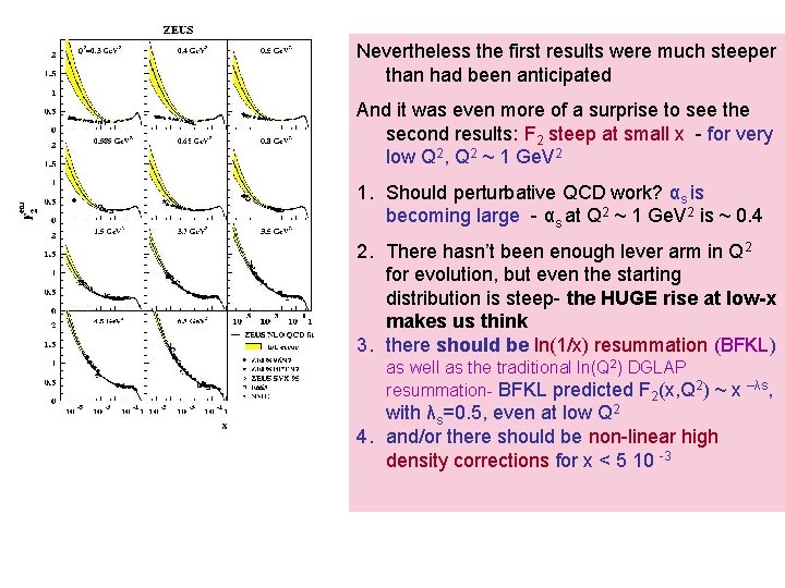
Nevertheless the first results were much steeper than had been anticipated And it was even more of a surprise to see the second results: F 2 steep at small x - for very low Q 2, Q 2 ~ 1 Ge. V 2 1. Should perturbative QCD work? αs is becoming large - αs at Q 2 ~ 1 Ge. V 2 is ~ 0. 4 2. There hasn’t been enough lever arm in Q 2 for evolution, but even the starting distribution is steep- the HUGE rise at low-x makes us think 3. there should be ln(1/x) resummation (BFKL) as well as the traditional ln(Q 2) DGLAP resummation- BFKL predicted F 2(x, Q 2) ~ x with λs=0. 5, even at low Q 2 4. and/or there should be non-linear high density corrections for x < 5 10 -3 –λs,

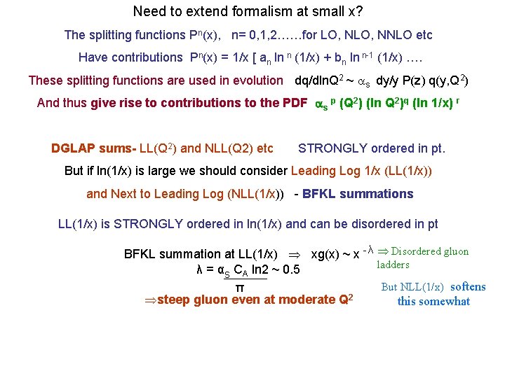
Need to extend formalism at small x? The splitting functions Pn(x), n= 0, 1, 2……for LO, NNLO etc Have contributions Pn(x) = 1/x [ an ln n (1/x) + bn ln n-1 (1/x) …. These splitting functions are used in evolution dq/dln. Q 2 ~ s dy/y P(z) q(y, Q 2) And thus give rise to contributions to the PDF s p (Q 2) (ln Q 2)q (ln 1/x) r DGLAP sums- LL(Q 2) and NLL(Q 2) etc STRONGLY ordered in pt. But if ln(1/x) is large we should consider Leading Log 1/x (LL(1/x)) and Next to Leading Log (NLL(1/x)) - BFKL summations LL(1/x) is STRONGLY ordered in ln(1/x) and can be disordered in pt BFKL summation at LL(1/x) xg(x) ~ x -λ Disordered gluon ladders λ = αs CA ln 2 ~ 0. 5 But NLL(1/x) softens π steep gluon even at moderate Q 2 this somewhat

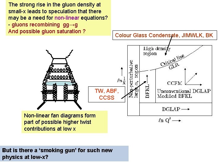
The strong rise in the gluon density at small-x leads to speculation that there may be a need for non-linear equations? - gluons recombining gg→g And possible gluon saturation ? Colour Glass Condensate, JIMWLK, BK TW, ABF, CCSS Non-linear fan diagrams form part of possible higher twist contributions at low x But is there a ‘smoking gun’ for such new physics at low-x?

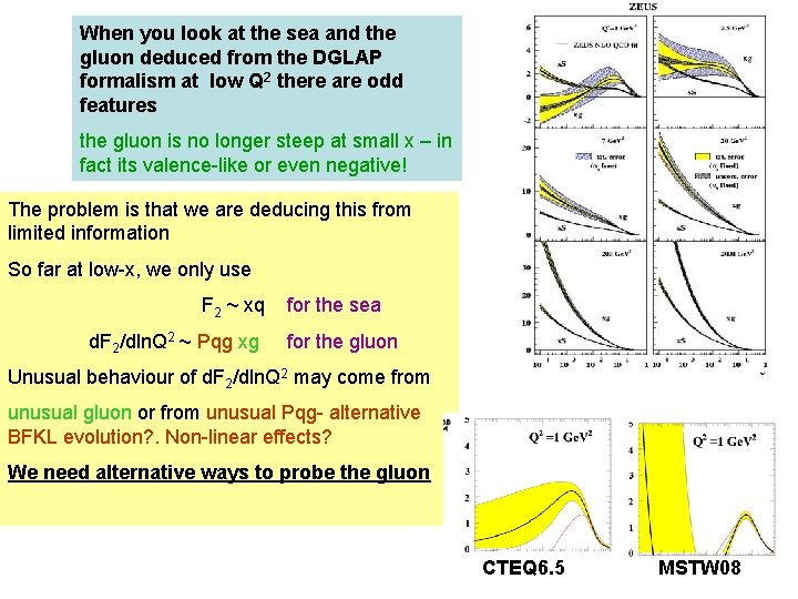
When you look at the sea and the gluon deduced from the DGLAP formalism at low Q 2 there are odd features the gluon is no longer steep at small x – in fact its valence-like or even negative! The problem is that we are deducing this from limited information So far at low-x, we only use F 2 ~ xq d. F 2/dln. Q 2 ~ Pqg xg for the sea for the gluon Unusual behaviour of d. F 2/dln. Q 2 may come from unusual gluon or from unusual Pqg- alternative BFKL evolution? . Non-linear effects? We need alternative ways to probe the gluon CTEQ 6. 5 MSTW 08

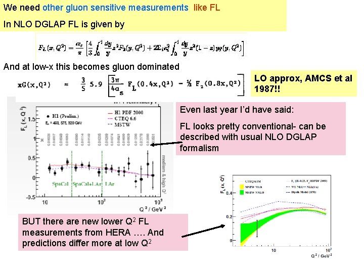
We need other gluon sensitive measurements like FL In NLO DGLAP FL is given by And at low-x this becomes gluon dominated LO approx, AMCS et al 1987!! Even last year I’d have said: FL looks pretty conventional- can be described with usual NLO DGLAP formalism BUT there are new lower Q 2 FL measurements from HERA …. And predictions differ more at low Q 2

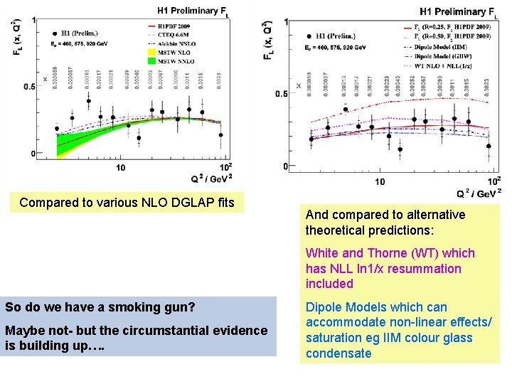
Compared to various NLO DGLAP fits And compared to alternative theoretical predictions: White and Thorne (WT) which has NLL ln 1/x resummation included So do we have a smoking gun? Maybe not- but the circumstantial evidence is building up…. Dipole Models which can accommodate non-linear effects/ saturation eg IIM colour glass condensate

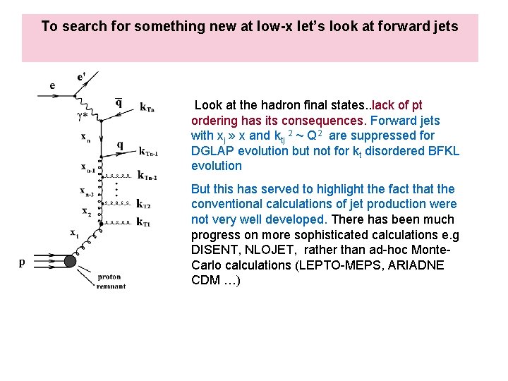
To search for something new at low-x let’s look at forward jets Look at the hadron final states. . lack of pt ordering has its consequences. Forward jets with xj » x and ktj 2 ~ Q 2 are suppressed for DGLAP evolution but not for kt disordered BFKL evolution But this has served to highlight the fact that the conventional calculations of jet production were not very well developed. There has been much progress on more sophisticated calculations e. g DISENT, NLOJET, rather than ad-hoc Monte. Carlo calculations (LEPTO-MEPS, ARIADNE CDM …)

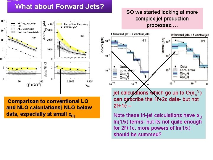
What about Forward Jets? Comparison to conventional LO and NLO calculations- NLO below data, especially at small x. Bj SO we started looking at more complex jet production processes…. jet calculations which go up to O(αs 3 ) can describe the 1 f+2 c data- but not 2 f+1 c – Note these tri-jet calculations have αS ln(1/x) terms- but its not quite enough for 2 f+1 c. . more powers of ln(1/x) should be summed?

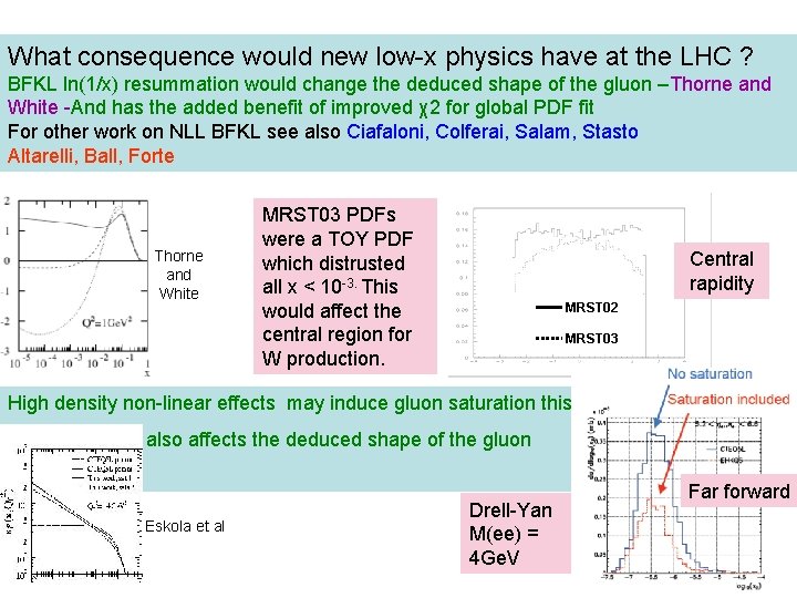
What consequence would new low-x physics have at the LHC ? BFKL ln(1/x) resummation would change the deduced shape of the gluon –Thorne and White -And has the added benefit of improved χ2 for global PDF fit For other work on NLL BFKL see also Ciafaloni, Colferai, Salam, Stasto Altarelli, Ball, Forte Thorne and White MRST 03 PDFs were a TOY PDF which distrusted all x < 10 -3. This would affect the central region for W production. Central rapidity MRST 02 MRST 03 High density non-linear effects may induce gluon saturation this also affects the deduced shape of the gluon Eskola et al Drell-Yan M(ee) = 4 Ge. V Far forward

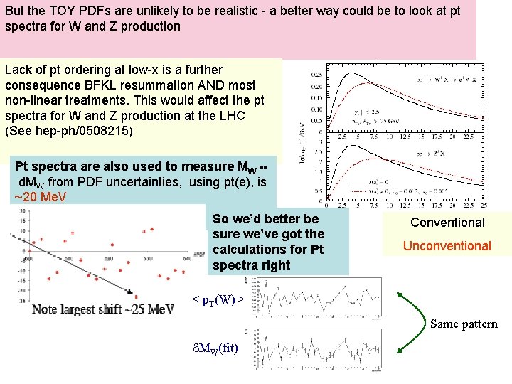
But the TOY PDFs are unlikely to be realistic - a better way could be to look at pt spectra for W and Z production Lack of pt ordering at low-x is a further consequence BFKL resummation AND most non-linear treatments. This would affect the pt spectra for W and Z production at the LHC (See hep-ph/0508215) Pt spectra are also used to measure MW -d. MW from PDF uncertainties, using pt(e), is ~20 Me. V So we’d better be sure we’ve got the calculations for Pt spectra right Conventional Unconventional < p. T(W) > Same pattern d. MW(fit)

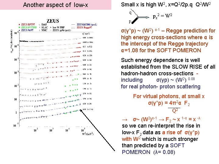
Another aspect of low-x Small x is high W 2, x=Q 2/2 p. q Q 2/W 2 q p px 2 = W 2 σ(γ*p) ~ (W 2) α-1 – Regge prediction for high energy cross-sections where α is the intercept of the Regge trajectory α=1. 08 for the SOFT POMERON Such energy dependence is well established from the SLOW RISE of all hadron-hadron cross-sections including σ(γp) ~ (W 2) 0. 08 for real photon- proton scattering For virtual photons, at small x σ(γ*p) = 4π2α F 2 Q 2 → σ~ (W 2)α-1 → F 2 ~ x 1 -α = x -λ so we can re-interpret the rise in low-x F 2 data as a rise of σ(γ*p) with W 2 which is much stronger than predicted by a SOFT POMERON (λ= 0. 08)

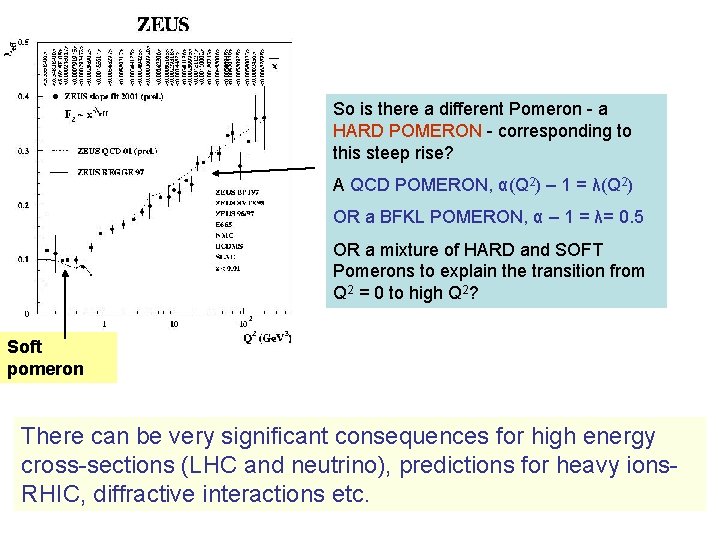
So is there a different Pomeron - a HARD POMERON - corresponding to this steep rise? A QCD POMERON, α(Q 2) – 1 = λ(Q 2) OR a BFKL POMERON, α – 1 = λ= 0. 5 OR a mixture of HARD and SOFT Pomerons to explain the transition from Q 2 = 0 to high Q 2? Soft pomeron There can be very significant consequences for high energy cross-sections (LHC and neutrino), predictions for heavy ions. RHIC, diffractive interactions etc.

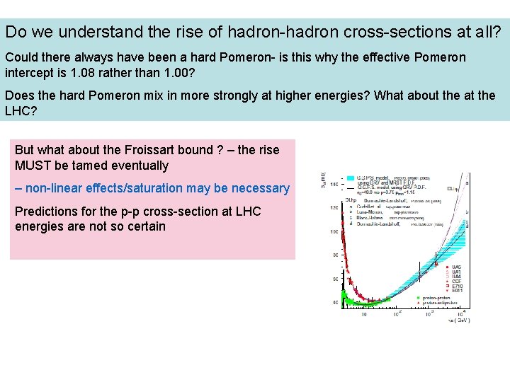
Do we understand the rise of hadron-hadron cross-sections at all? Could there always have been a hard Pomeron- is this why the effective Pomeron intercept is 1. 08 rather than 1. 00? Does the hard Pomeron mix in more strongly at higher energies? What about the at the LHC? But what about the Froissart bound ? – the rise MUST be tamed eventually – non-linear effects/saturation may be necessary Predictions for the p-p cross-section at LHC energies are not so certain

Summary • There is evidence that all is not well with conventional QCD calculations at low-x • Trouble sets in for x < 10 -2 • Which means that SM calculations may not look as we expect even in the central rapidity region at the LHC • These effects can be explicitly studied in the forward detectors/ in heavy ion collisions/ in diffractive processes

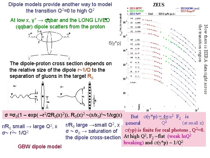
Dipole models provide another way to model the transition Q 2=0 to high Q 2 б(γ*p) The dipole-proton cross section depends on the relative size of the dipole r~1/Q to the separation of gluons in the target R 0 σ =σ0(1 – exp( –r 2/2 R 0(x)2)), R 0(x)2 ~(x/x 0)λ~1/xg(x) r/R 0 small → large Q 2, x σ~ r 2~ 1/Q 2 GBW dipole model Now there is HERA data right across the transition region At low x, γ* → qqbar and the LONG LIVED (qqbar) dipole scatters from the proton But (g*p) = 4 p 2 F 2 is Q 2 (at small x) r/R 0 large →small Q 2, x general 2 σ ~ σ0 → saturation of (gp) is finite for real photons , Q =0. 2 2 the dipole cross-section At high Q , F 2 ~flat (weak ln. Q breaking) and (g*p) ~ 1/Q 2

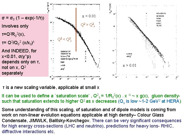
x < 0. 01 σ = σ0 (1 – exp(-1/τ)) Q 2 > Q 2 s Involves only τ=Q 2 R 02(x), τ= Q 2/Q 02 (x/x 0 )λ Q 2 < Q 2 s And INDEED, for x<0. 01, σ(γ*p) depends only on τ, not on x, Q 2 separately x > 0. 01 τ is a new scaling variable, applicable at small x It can be used to define a `saturation scale’ , Q 2 s = 1/R 02(x). x -λ ~ x g(x), gluon densitysuch that saturation extends to higher Q 2 as x decreases (Qs is low ~1 -2 Ge. V 2 at HERA) Some understanding of this scaling, of saturation and of dipole models is coming from work on non-linear evolution equations applicable at high density– Colour Glass Condensate, JIMWLK, Balitsky-Kovchegov. There can be very significant consequences for high energy cross-sections (LHC and neutrino), predictions for heavy ions- RHIC, diffractive interactions etc.

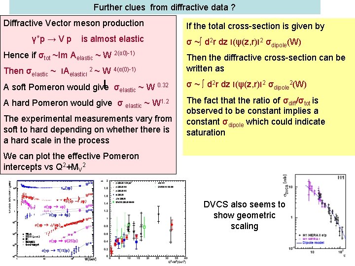
Further clues from diffractive data ? Diffractive Vector meson production γ*p → V p is almost elastic Hence if σtot ~Im Aelastic ~ W 2(α 0)-1) If the total cross-section is given by σ ~∫ d 2 r dz (׀ ψ(z, r) ׀ 2 σdipole(W) Then σelastic ~ ׀ Aelastic ׀ 2 ~ W 4(α(0)-1) Then the diffractive cross-section can be written as A soft Pomeron would give σelastic ~ W 0. 32 σ ~ ∫ d 2 r dz (׀ ψ(z, r) ׀ 2 σdipole 2(W) A hard Pomeron would give σ elastic ~ W 1. 2 The fact that the ratio of σdiff/σtot is observed to be constant implies a constant σdipole which could indicate saturation The experimental measurements vary from soft to hard depending on whethere is a hard scale in the process We can plot the effective Pomeron intercepts vs Q 2+MV 2 DVCS also seems to show geometric scaling

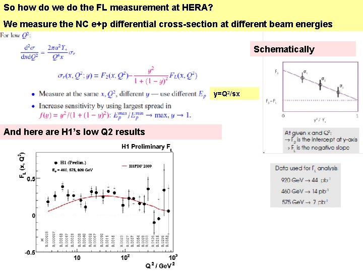
So how do we do the FL measurement at HERA? We measure the NC e+p differential cross-section at different beam energies Schematically y=Q 2/sx And here are H 1’s low Q 2 results

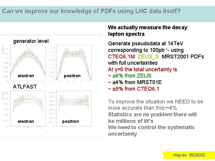
Can we improve our knowledge of PDFs using LHC data itself? We actually measure the decay lepton spectra generator level electron positron ATLFAST electron positron Generate pseudodata at 14 Te. V corresponding to 100 pb-1 - using CTEQ 6. 1 M ZEUS_S MRST 2001 PDFs with full uncertainties At y=0 the total uncertainty is ~ ± 6% from ZEUS ~ ± 4% from MRST 01 E ~ ± 8% from CTEQ 6. 1 To improve the situation we NEED to be more accurate than this: ~4% Statistics are no problem there will be millions of W’s We need to control the systematic uncertainty Hep-ex: 0509002

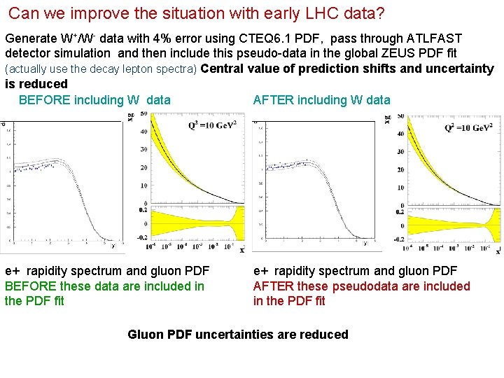
Can we improve the situation with early LHC data? Generate W+/W- data with 4% error using CTEQ 6. 1 PDF, pass through ATLFAST detector simulation and then include this pseudo-data in the global ZEUS PDF fit (actually use the decay lepton spectra) Central value of prediction shifts and uncertainty is reduced BEFORE including W data AFTER including W data e+ rapidity spectrum and gluon PDF BEFORE these data are included in the PDF fit e+ rapidity spectrum and gluon PDF AFTER these pseudodata are included in the PDF fit Gluon PDF uncertainties are reduced

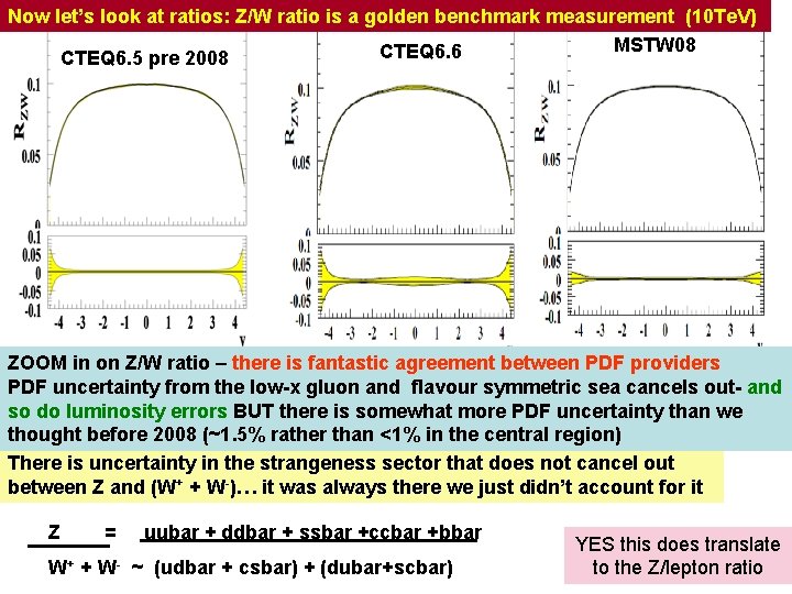
Now let’s look at ratios: Z/W ratio is a golden benchmark measurement (10 Te. V) MSTW 08 CTEQ 6. 6 CTEQ 6. 5 pre 2008 ZOOM in on Z/W ratio – there is fantastic agreement between PDF providers PDF uncertainty from the low-x gluon and flavour symmetric sea cancels out- and so do luminosity errors BUT there is somewhat more PDF uncertainty than we thought before 2008 (~1. 5% rather than <1% in the central region) There is uncertainty in the strangeness sector that does not cancel out between Z and (W+ + W-)… it was always there we just didn’t account for it Z = uubar + ddbar + ssbar +ccbar +bbar W+ + W- ~ (udbar + csbar) + (dubar+scbar) YES this does translate to the Z/lepton ratio

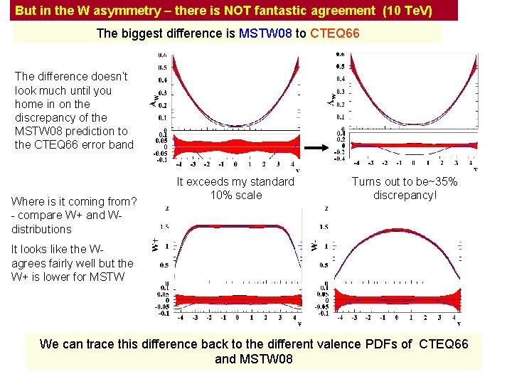
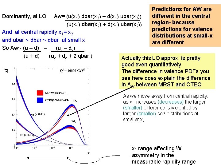
But in the W asymmetry – there is NOT fantastic agreement (10 Te. V) The biggest difference is MSTW 08 to CTEQ 66 The difference doesn’t look much until you home in on the discrepancy of the MSTW 08 prediction to the CTEQ 66 error band Where is it coming from? - compare W+ and Wdistributions It exceeds my standard 10% scale Turns out to be~35% discrepancy! It looks like the Wagrees fairly well but the W+ is lower for MSTW We can trace this difference back to the different valence PDFs of CTEQ 66 and MSTW 08

Dominantly, at LO Predictions for AW are different in the central region- because predictions for valence distributions at small-x are different Aw= (u(x 1) dbar(x 2) – d(x 1) ubar(x 2)) (u(x 1) dbar(x 2) + d(x 1) ubar(x 2)) And at central rapidity x 1= x 2 and ubar ~ dbar ~ qbar at small x So Aw~ (u – d) = (uv – dv) (u + d) (uv + dv + 2 qbar ) Actually this LO approx. is pretty good even quantitatively The difference in valence PDFs you see here does explain the difference in AW between MRST and CTEQ As we move away from central rapidity: as x 1 increases (decreases) the larger (smaller) difference is weighted by larger (smaller) sea distributions at smaller x 2 x- range affecting W asymmetry in the measurable rapidity range