Linear Regression Used to determine how the outcome
- Slides: 9

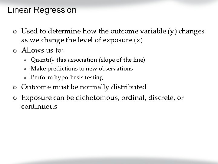
Linear Regression Used to determine how the outcome variable (y) changes as we change the level of exposure (x) Allows us to: l l l Quantify this association (slope of the line) Make predictions to new observations Perform hypothesis testing Outcome must be normally distributed Exposure can be dichotomous, ordinal, discrete, or continuous

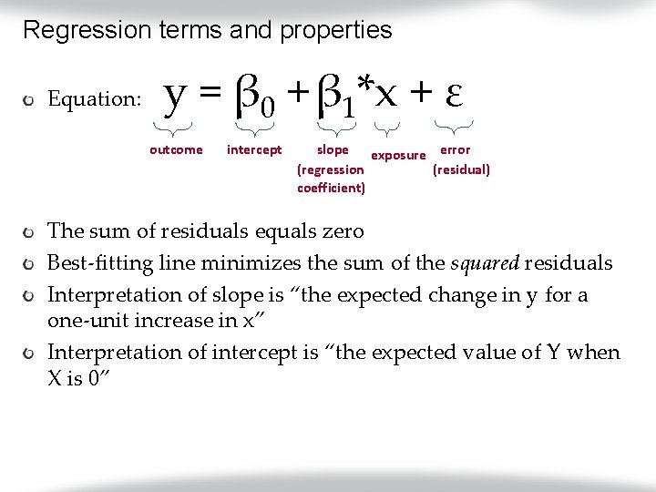
Regression terms and properties Equation: y = β 0 + β 1*x + ε outcome intercept slope exposure error (residual) (regression coefficient) The sum of residuals equals zero Best-fitting line minimizes the sum of the squared residuals Interpretation of slope is “the expected change in y for a one-unit increase in x” Interpretation of intercept is “the expected value of Y when X is 0”

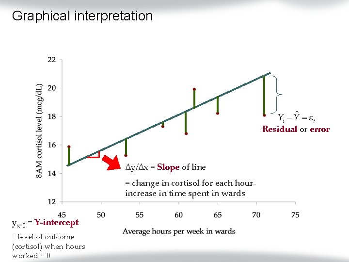
Graphical interpretation Residual or error ∆y/∆x = Slope of line = change in cortisol for each hourincrease in time spent in wards yx=0 = Y-intercept = level of outcome (cortisol) when hours worked = 0

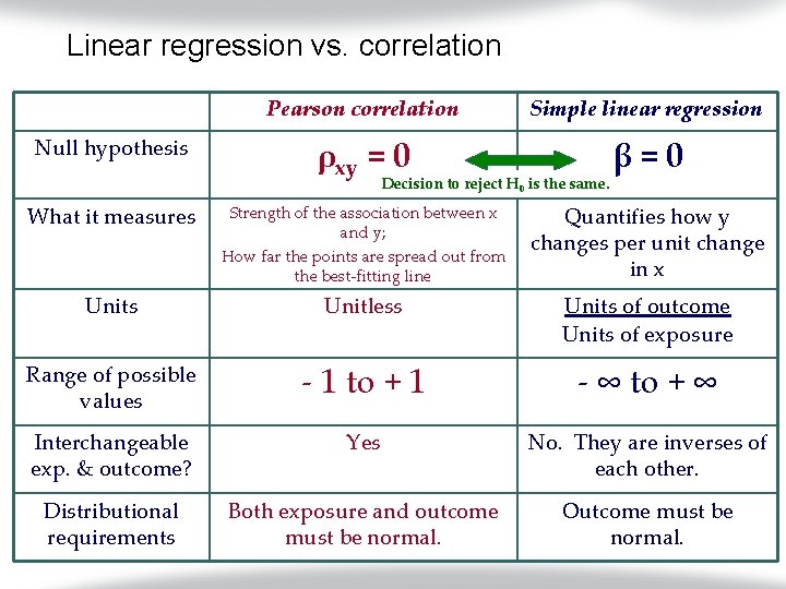
Linear regression vs. correlation Pearson correlation Simple linear regression ρxy = 0 β=0 What it measures Strength of the association between x and y; How far the points are spread out from the best-fitting line Quantifies how y changes per unit change in x Units Unitless Units of outcome Units of exposure Range of possible values - 1 to + 1 - ∞ to + ∞ Interchangeable exp. & outcome? Yes No. They are inverses of each other. Distributional requirements Both exposure and outcome must be normal. Outcome must be normal. Null hypothesis Decision to reject H 0 is the same.

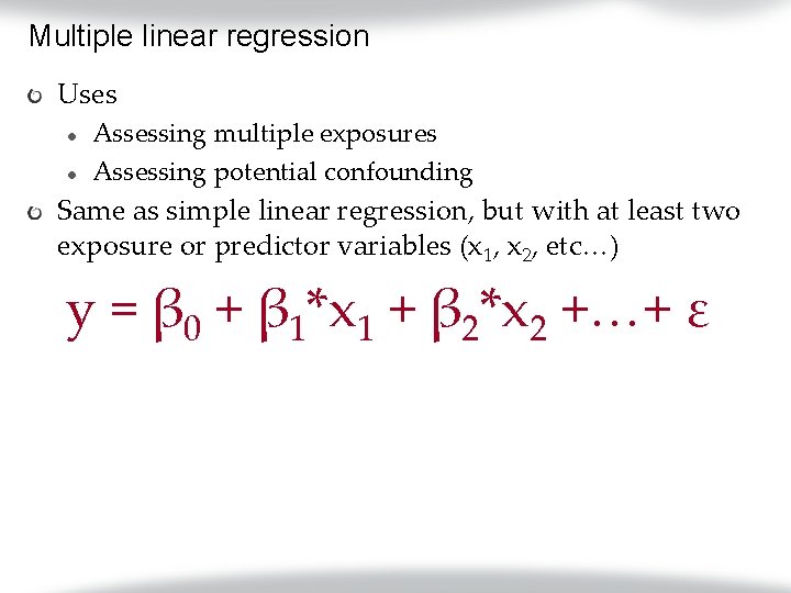
Multiple linear regression Uses l l Assessing multiple exposures Assessing potential confounding Same as simple linear regression, but with at least two exposure or predictor variables (x 1, x 2, etc…) y = β 0 + β 1*x 1 + β 2*x 2 +…+ ε

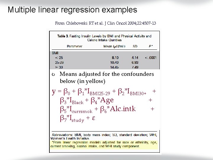
Multiple linear regression examples From Chlebowski RT et al. J Clin Oncol 2004; 22: 4507 -13 Means adjusted for the confounders below (in yellow) y = β 0 + β 1*IBMI 25 -29 + β 2*IBMI 30+ + β 3*IBlack + β 4*Age + β 5*Icurrsmok + β 6*Alc. intk + β 7*Istudy + ε

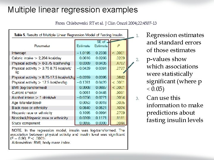
Multiple linear regression examples From Chlebowski RT et al. J Clin Oncol 2004; 22: 4507 -13 1. 2. 3. Regression estimates and standard errors of those estimates p-values show which associations were statistically significant (where p < 0. 05) Can use this information to make predictions about fasting insulin levels

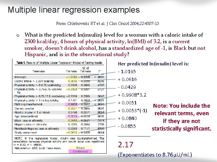
Multiple linear regression examples From Chlebowski RT et al. J Clin Oncol 2004; 22: 4507 -13 What is the predicted ln(insulin) level for a woman with a caloric intake of 2300 kcal/day, 4 hours of physical activity, ln(BMI) of 3. 2, is a current smoker, doesn’t drink alcohol, has a standardized age of -1, is Black but not Hispanic, and is in the observational study? Her predicted ln(insulin) level is: - 1. 0195 + 0. 0616 - 0. 0429 + 0. 9908*3. 2 + 0. 0051 Note: You include the + 0. 0053*(-1) relevant terms, even + 0. 0840 if they are not - 0. 0855 statistically significant. ______ Binary Continuous 2. 17 (Exponentiates to 8. 76μU/m. L)

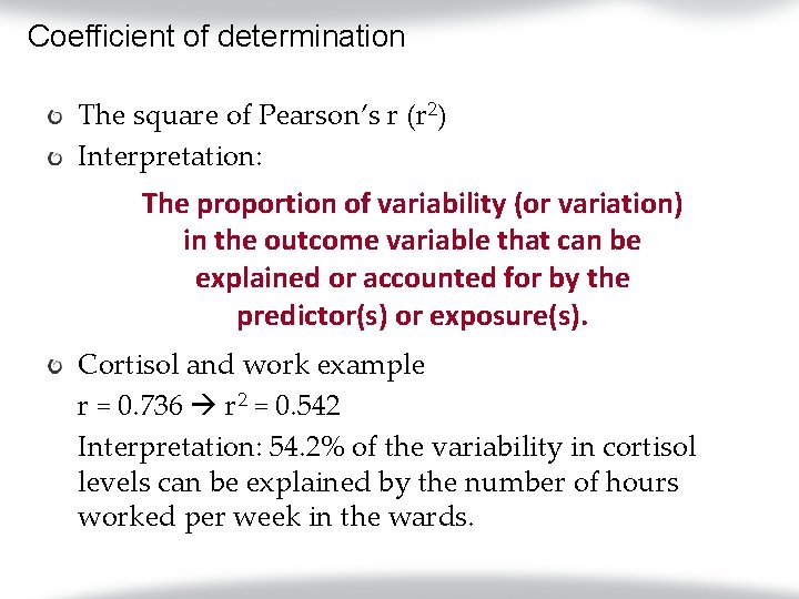
Coefficient of determination The square of Pearson’s r (r 2) Interpretation: The proportion of variability (or variation) in the outcome variable that can be explained or accounted for by the predictor(s) or exposure(s). Cortisol and work example r = 0. 736 r 2 = 0. 542 Interpretation: 54. 2% of the variability in cortisol levels can be explained by the number of hours worked per week in the wards.