Lecture 15 Fractals Scaling and the Hurst Exponent

Lecture 15 Fractals, Scaling and the Hurst Exponent John Rundle Econophysics PHYS 250

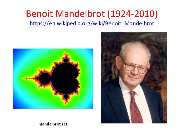
Benoit Mandelbrot (1924 -2010) https: //en. wikipedia. org/wiki/Benoit_Mandelbrot set

Benoit Mandelbrot (1924 -2010) https: //en. wikipedia. org/wiki/Benoit_Mandelbrot • Benoit B.  Mandelbrot  (20 November 1924 – 14 October 2010) was a Polish-born, French and American mathematician with broad interests in the practical sciences, especially regarding what he labeled as "the art of roughness" of physical phenomena and "the uncontrolled element in life. " • He is recognized for his contribution to the field of fractal geometry, which included coining the word "fractal'", as well as developing a theory of "roughness and self-similarity" in nature. • In 1936, while he was a child, Mandelbrot's family migrated to France. • After World War II ended, Mandelbrot studied mathematics, graduating from universities in Paris and the United States and receiving a master's degree in aeronautics from the California Institute of Technology. • He spent most of his career in both the United States and France, having dual French and American citizenship. In 1958, he began a 35 -year career at IBM, where he became an IBM Fellow, and periodically took leaves of absence to teach at Harvard University. • At Harvard, following the publication of his study of U. S. commodity markets in relation to cotton futures, he taught economics and applied sciences.

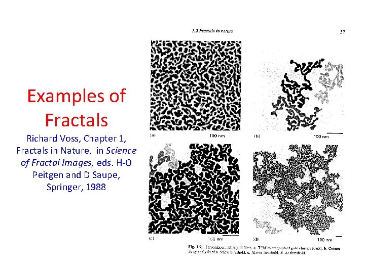
Examples of Fractals Richard Voss, Chapter 1, Fractals in Nature, in Science of Fractal Images, eds. H-O Peitgen and D Saupe, Springer, 1988

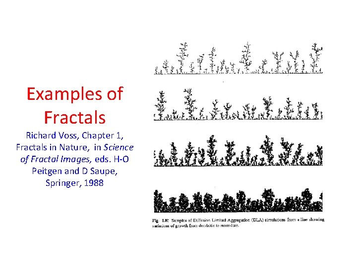
Examples of Fractals Richard Voss, Chapter 1, Fractals in Nature, in Science of Fractal Images, eds. H-O Peitgen and D Saupe, Springer, 1988

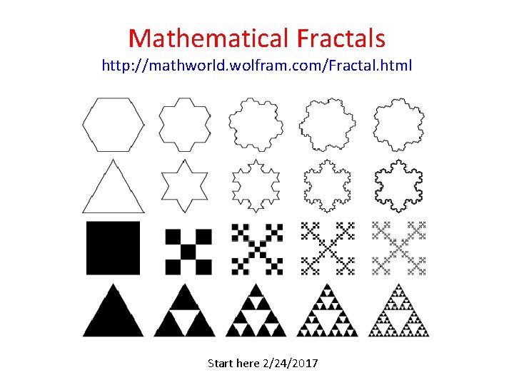
Mathematical Fractals http: //mathworld. wolfram. com/Fractal. html Start here 2/24/2017

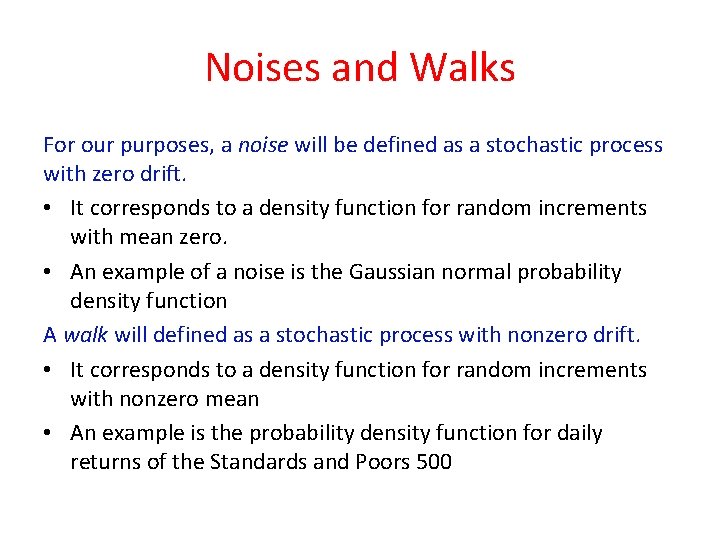
Noises and Walks For our purposes, a noise will be defined as a stochastic process with zero drift. • It corresponds to a density function for random increments with mean zero. • An example of a noise is the Gaussian normal probability density function A walk will defined as a stochastic process with nonzero drift. • It corresponds to a density function for random increments with nonzero mean • An example is the probability density function for daily returns of the Standards and Poors 500

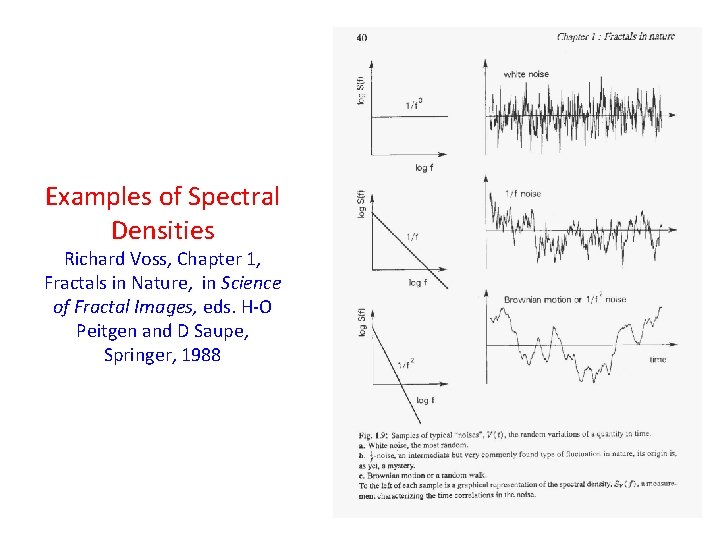
Examples of Spectral Densities Richard Voss, Chapter 1, Fractals in Nature, in Science of Fractal Images, eds. H-O Peitgen and D Saupe, Springer, 1988

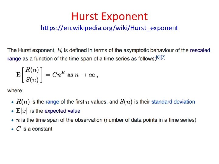
Hurst Exponent (or “Index”) https: //en. wikipedia. org/wiki/Hurst_exponent • The Hurst exponent is used as a measure of long-term memory of time series. • It relates to the autocorrelations of the time series, and the rate at which these decrease as the lag between pairs of values increases. • Studies involving the Hurst exponent were originally developed in hydrology for the practical matter of determining optimum dam sizing for the Nile river's volatile rain and drought conditions that had been observed over a long period of time. • The name "Hurst exponent", or "Hurst coefficient", derives from Harold Edwin Hurst (1880– 1978), who was the lead researcher in these studies • The use of the standard notation H for the coefficient relates to his name also.

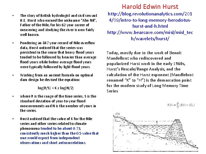
Harold Edwin Hurst • The story of British hydrologist and civil servant H. E. Hurst who earned the nickname “Abu Nil”, Father of the Nile, for his 62 year career of measuring and studying the river is now fairly well known. • Pondering an 847 year record of Nile overflow data, Hurst noticed that the series was persistent in the sense that heavy flood years tended to be followed by heavier than average flood years while below average flood years were typically followed by light flood years. • Working from an ancient formula on optimal dam design he devised the equation: log(R/S) = K x log(N/2) • where R is the range of the time series, S is the standard deviation of year-to-year flood measurements and N is the number of years in the series. • Hurst noticed that the value of K for the Nile series and other series related to climate phenomena tended to be about 0. 73, consistently much higher than the 0. 5 value that one would expect from independent observations and short autocorrelations. http: //blog. revolutionanalytics. com/201 4/09/intro-to-long-memory-herodotushurst-and-h. html http: //www. bearcave. com/misl_tec h/wavelets/hurst/ Today, mostly due to the work of Benoit Mandelbrot who rediscovered and popularized Hurst work in the early 1960 s, Hurst’s Rescale/Range Analysis, and the calculation of the Hurst exponent (Mandlebrot renamed “K” to “H”) is the demarcation point for the modern study of Long Memory Time Series

Hurst Exponent https: //en. wikipedia. org/wiki/Hurst_exponent

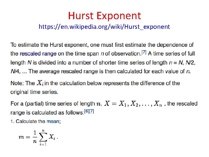
Hurst Exponent https: //en. wikipedia. org/wiki/Hurst_exponent

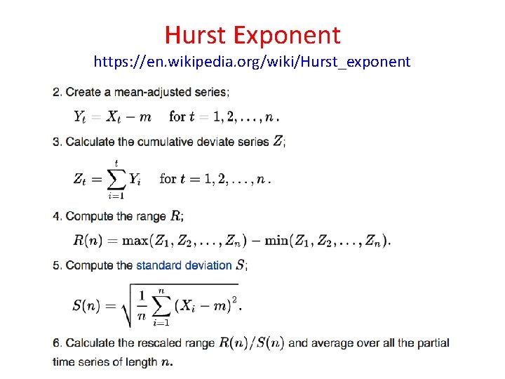
Hurst Exponent https: //en. wikipedia. org/wiki/Hurst_exponent

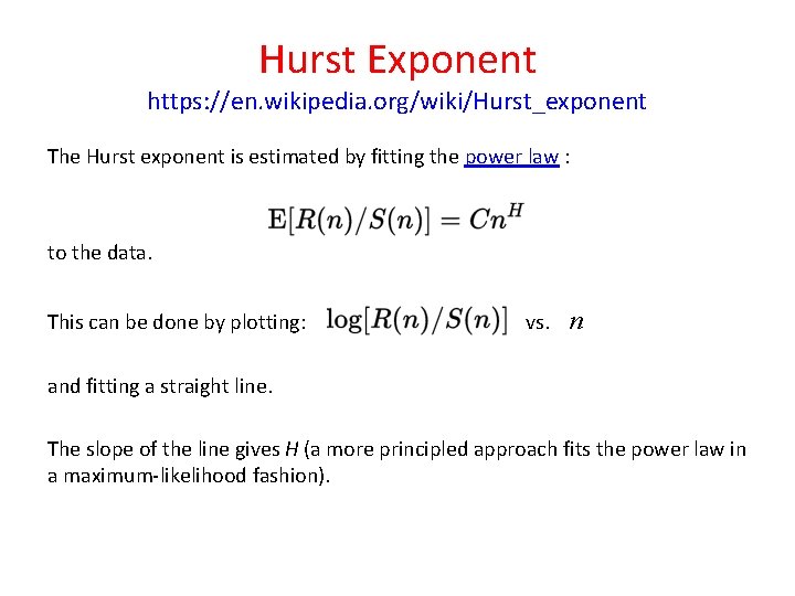
Hurst Exponent https: //en. wikipedia. org/wiki/Hurst_exponent The Hurst exponent is estimated by fitting the power law : to the data. This can be done by plotting: vs. n and fitting a straight line. The slope of the line gives H (a more principled approach fits the power law in a maximum-likelihood fashion).

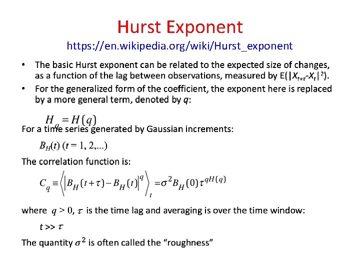
Hurst Exponent https: //en. wikipedia. org/wiki/Hurst_exponent •

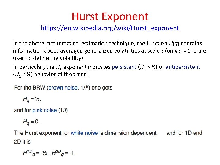
Hurst Exponent https: //en. wikipedia. org/wiki/Hurst_exponent In the above mathematical estimation technique, the function H(q) contains information about averaged generalized volatilities at scale τ (only q = 1, 2 are used to define the volatility). In particular, the H 1 exponent indicates persistent (H 1 > ½) or antipersistent (H 1 < ½) behavior of the trend.

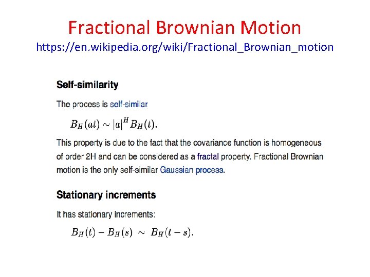
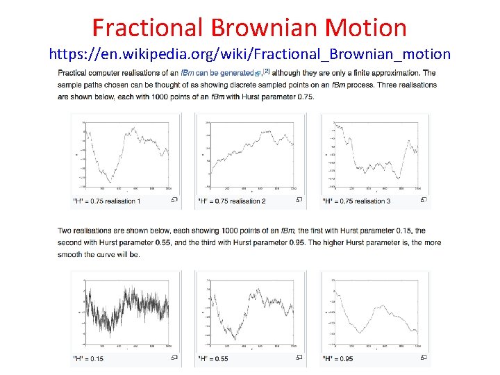
Fractional Brownian Motion https: //en. wikipedia. org/wiki/Fractional_Brownian_motion (Here BH(t) is the walk)

Fractional Brownian Motion https: //en. wikipedia. org/wiki/Fractional_Brownian_motion

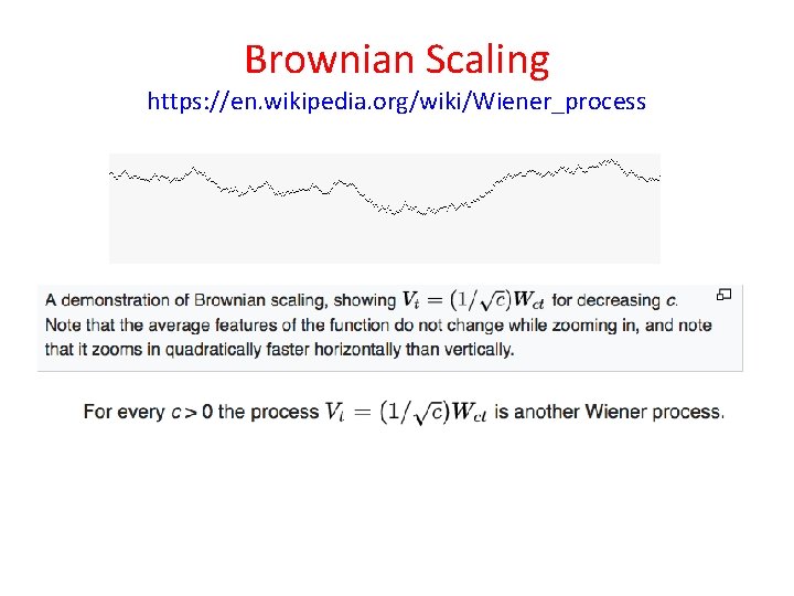
Brownian Scaling https: //en. wikipedia. org/wiki/Wiener_process

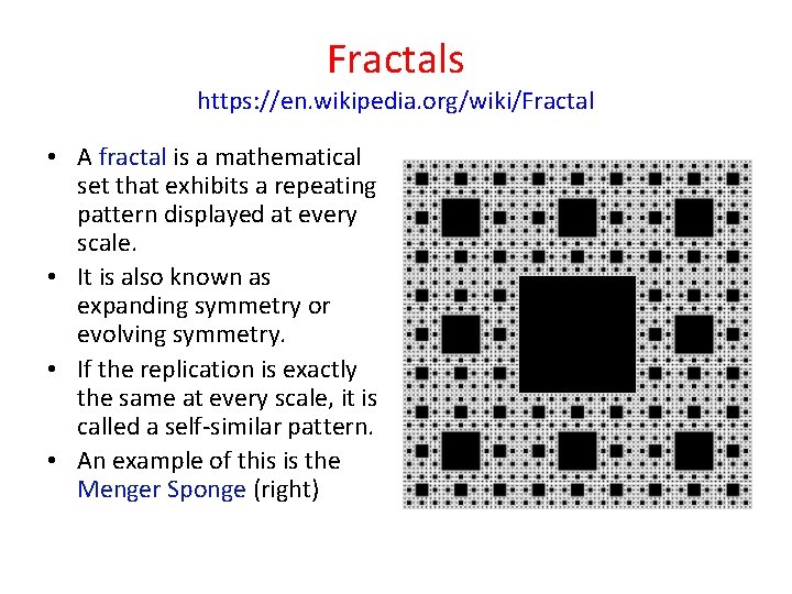
Fractals https: //en. wikipedia. org/wiki/Fractal • A fractal is a mathematical set that exhibits a repeating pattern displayed at every scale. • It is also known as expanding symmetry or evolving symmetry. • If the replication is exactly the same at every scale, it is called a self-similar pattern. • An example of this is the Menger Sponge (right)

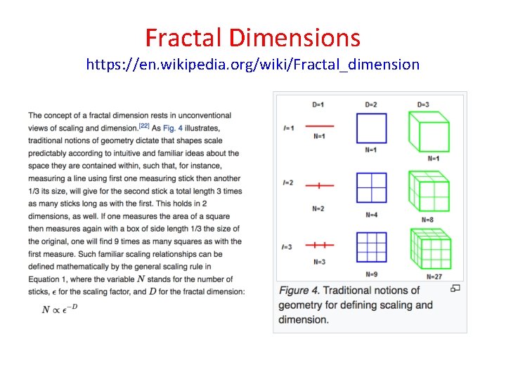
Fractal Dimensions https: //en. wikipedia. org/wiki/Fractal_dimension • In mathematics, more specifically in fractal geometry, a fractal dimension is a ratio providing a statistical index of complexity comparing how detail in a pattern (strictly speaking, a fractal pattern) changes with the scale at which it is measured. • It has also been characterized as a measure of the space-filling capacity of a pattern that tells how a fractal scales differently from the space it is embedded in • A fractal dimension is generally not an integer. • An embedding dimension is an integer, however

Fractal Dimensions https: //en. wikipedia. org/wiki/Fractal_dimension

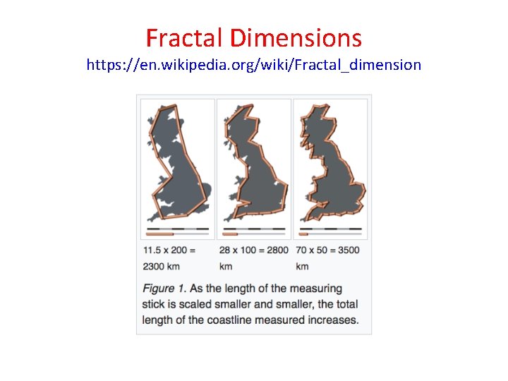
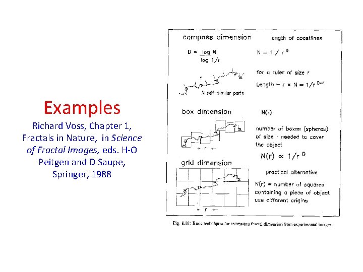
Fractal Dimensions https: //en. wikipedia. org/wiki/Fractal_dimension • The essential idea of "fractured" dimensions has a long history in mathematics, but the term itself was brought to the fore by Benoit Mandelbrot based on his 1967 paper on self-similarity in which he discussed fractional dimensions. • In that paper, Mandelbrot cited previous work by Lewis Fry Richardson describing the counter-intuitive notion that a coastline's measured length changes with the length of the measuring stick used (previous slide). • In terms of that notion, the fractal dimension of a coastline quantifies how the number of scaled measuring sticks required to measure the coastline changes with the scale applied to the stick. • There are several formal mathematical definitions of fractal dimension that build on this basic concept of change in detail with change in scale.

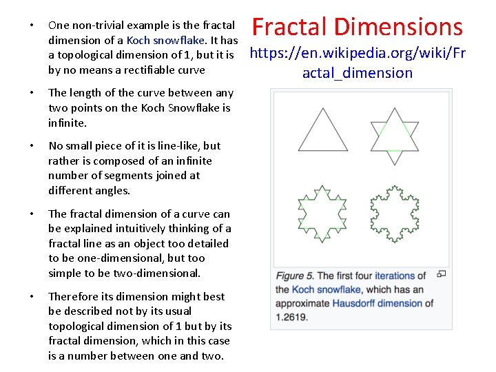
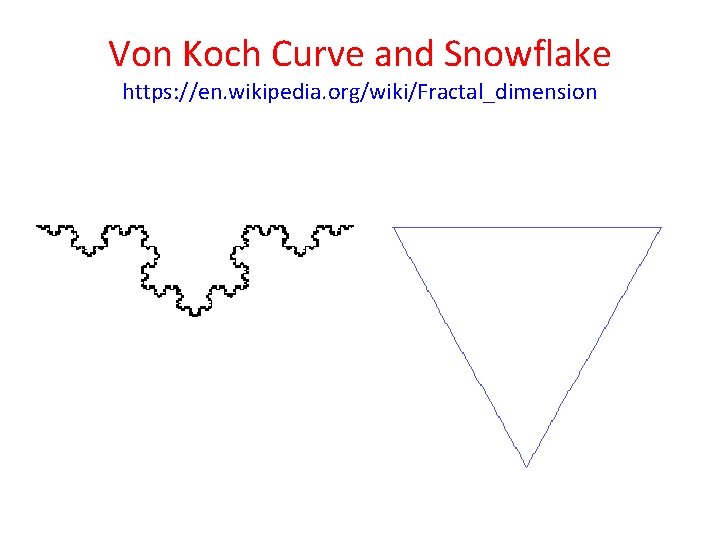
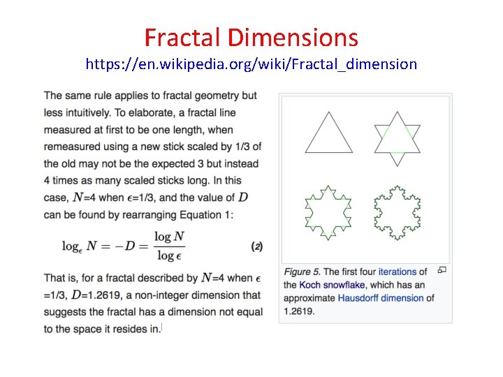
• One non-trivial example is the fractal dimension of a Koch snowflake. It has a topological dimension of 1, but it is by no means a rectifiable curve • The length of the curve between any two points on the Koch Snowflake is infinite. • No small piece of it is line-like, but rather is composed of an infinite number of segments joined at different angles. • The fractal dimension of a curve can be explained intuitively thinking of a fractal line as an object too detailed to be one-dimensional, but too simple to be two-dimensional. • Therefore its dimension might best be described not by its usual topological dimension of 1 but by its fractal dimension, which in this case is a number between one and two. Fractal Dimensions https: //en. wikipedia. org/wiki/Fr actal_dimension

Von Koch Curve and Snowflake https: //en. wikipedia. org/wiki/Fractal_dimension

Fractal Dimensions https: //en. wikipedia. org/wiki/Fractal_dimension

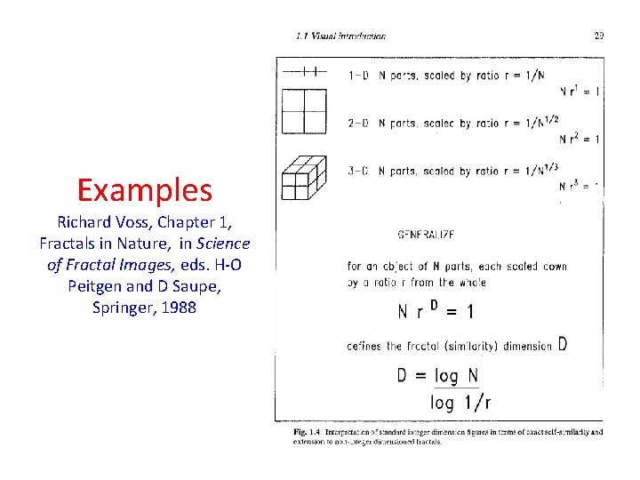
Examples Richard Voss, Chapter 1, Fractals in Nature, in Science of Fractal Images, eds. H-O Peitgen and D Saupe, Springer, 1988

Fractal Dimensions https: //en. wikipedia. org/wiki/Fractal_dimension

Examples Richard Voss, Chapter 1, Fractals in Nature, in Science of Fractal Images, eds. H-O Peitgen and D Saupe, Springer, 1988

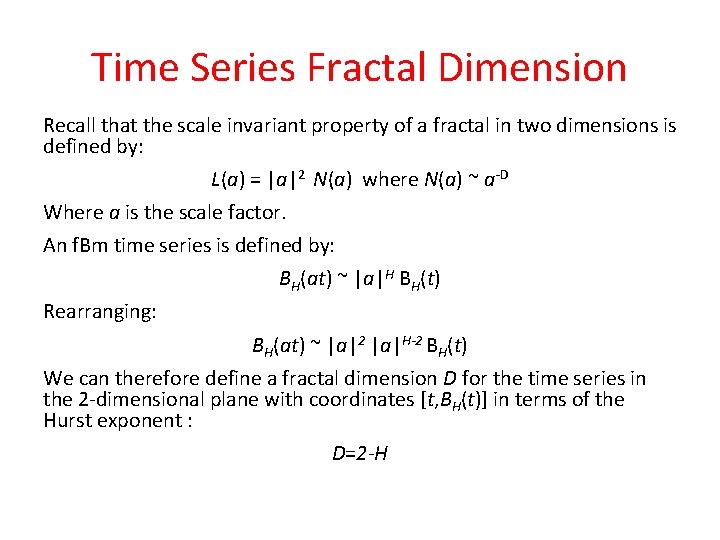
Time Series Fractal Dimension Recall that the scale invariant property of a fractal in two dimensions is defined by: L(a) = |a|2 N(a) where N(a) ~ a-D Where a is the scale factor. An f. Bm time series is defined by: BH(at) ~ |a|H BH(t) Rearranging: BH(at) ~ |a|2 |a|H-2 BH(t) We can therefore define a fractal dimension D for the time series in the 2 -dimensional plane with coordinates [t, BH(t)] in terms of the Hurst exponent : D=2 -H

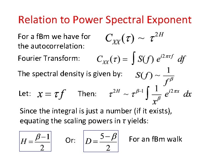
Relation to Power Spectral Exponent For a f. Bm we have for the autocorrelation: Fourier Transform: The spectral density is given by: Let: Then: Since the integral is just a number (if it exists), equating the scaling powers in τ yields: Or: For an f. Bm walk

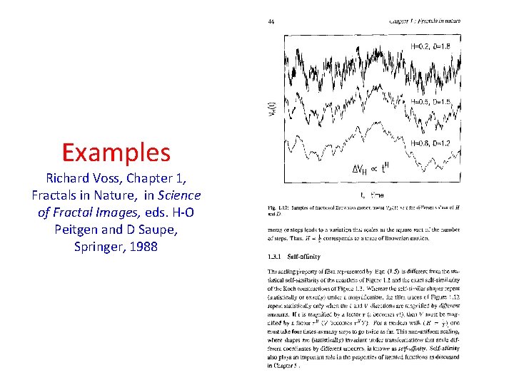
Examples Richard Voss, Chapter 1, Fractals in Nature, in Science of Fractal Images, eds. H-O Peitgen and D Saupe, Springer, 1988

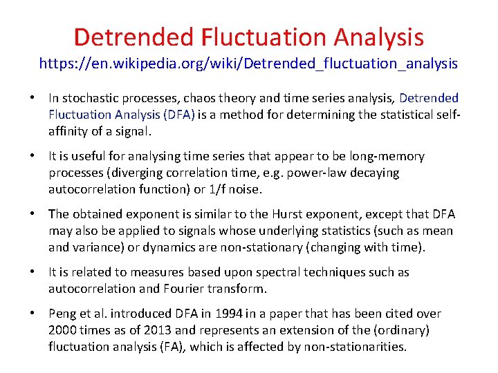
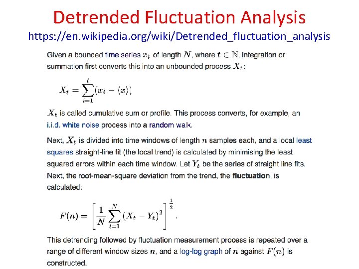
Detrended Fluctuation Analysis https: //en. wikipedia. org/wiki/Detrended_fluctuation_analysis • In stochastic processes, chaos theory and time series analysis, Detrended Fluctuation Analysis (DFA) is a method for determining the statistical selfaffinity of a signal. • It is useful for analysing time series that appear to be long-memory processes (diverging correlation time, e. g. power-law decaying autocorrelation function) or 1/f noise. • The obtained exponent is similar to the Hurst exponent, except that DFA may also be applied to signals whose underlying statistics (such as mean and variance) or dynamics are non-stationary (changing with time). • It is related to measures based upon spectral techniques such as autocorrelation and Fourier transform. • Peng et al. introduced DFA in 1994 in a paper that has been cited over 2000 times as of 2013 and represents an extension of the (ordinary) fluctuation analysis (FA), which is affected by non-stationarities.

Detrended Fluctuation Analysis https: //en. wikipedia. org/wiki/Detrended_fluctuation_analysis

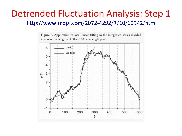
Detrended Fluctuation Analysis: Step 1 http: //www. mdpi. com/2072 -4292/7/10/12942/htm

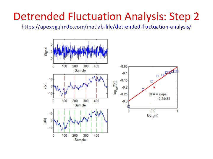
Detrended Fluctuation Analysis: Step 2 https: //apexpg. jimdo. com/matlab-file/detrended-fluctuation-analysis/

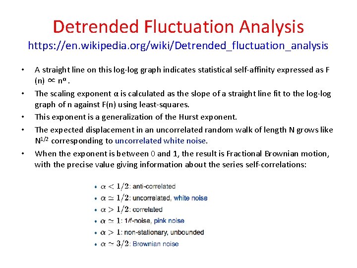
Detrended Fluctuation Analysis https: //en. wikipedia. org/wiki/Detrended_fluctuation_analysis • • • A straight line on this log-log graph indicates statistical self-affinity expressed as F (n) ∝ nα. The scaling exponent α is calculated as the slope of a straight line fit to the log-log graph of n against F(n) using least-squares. This exponent is a generalization of the Hurst exponent. The expected displacement in an uncorrelated random walk of length N grows like N 1/2 corresponding to uncorrelated white noise. When the exponent is between 0 and 1, the result is Fractional Brownian motion, with the precise value giving information about the series self-correlations:

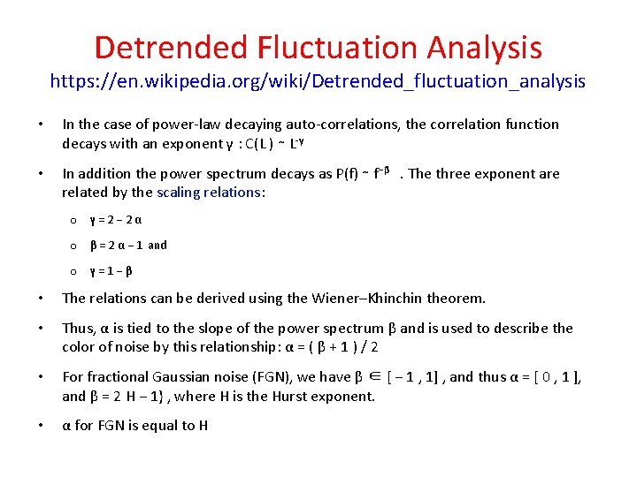
Detrended Fluctuation Analysis https: //en. wikipedia. org/wiki/Detrended_fluctuation_analysis • In the case of power-law decaying auto-correlations, the correlation function decays with an exponent γ : C(L ) ∼ L-γ • In addition the power spectrum decays as P(f) ∼ f−β . The three exponent are related by the scaling relations: o γ = 2 − 2 α o β = 2 α − 1 and o γ = 1 − β • The relations can be derived using the Wiener–Khinchin theorem. • Thus, α is tied to the slope of the power spectrum β and is used to describe the color of noise by this relationship: α = ( β + 1 ) / 2 • For fractional Gaussian noise (FGN), we have β ∈ [ − 1 , 1] , and thus α = [ 0 , 1 ], and β = 2 H − 1} , where H is the Hurst exponent. • α for FGN is equal to H