Lecture 11 Linearization 2 Linearization of a nonlinear

Lecture 11: Linearization 2. Linearization of a nonlinear function 3. Linearization of a nonlinear diff equation ME 431, Lecture 11 1. Introduction 1

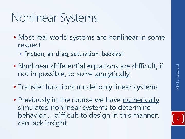
Nonlinear Systems • Most real world systems are nonlinear in some respect • Nonlinear differential equations are difficult, if not impossible, to solve analytically • Transfer functions model only linear systems • Previously in the course we have numerically simulated nonlinear systems to determine behavior … difficult to design in this manner, can lack insight ME 431, Lecture 11 • Friction, air drag, saturation, backlash 2

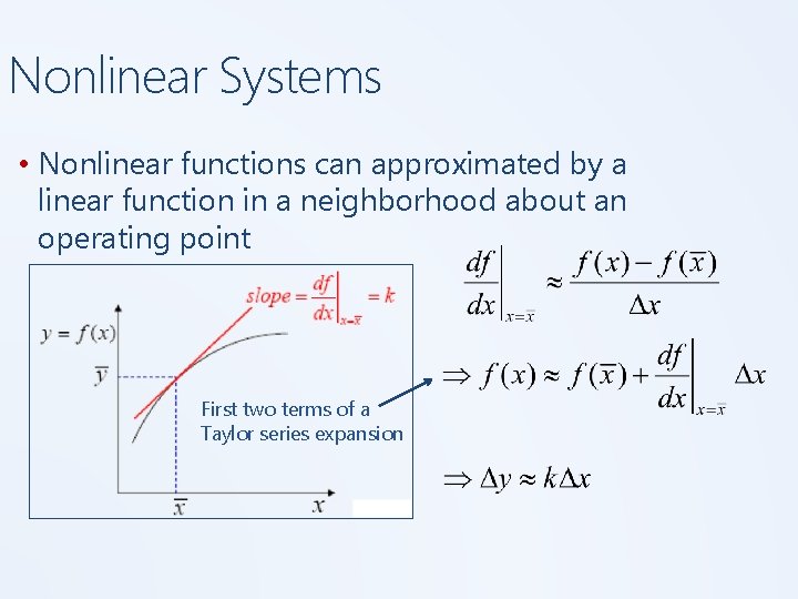
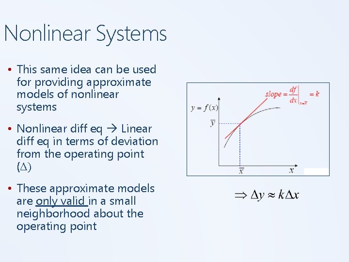
Nonlinear Systems • Nonlinear functions can approximated by a linear function in a neighborhood about an operating point First two terms of a Taylor series expansion

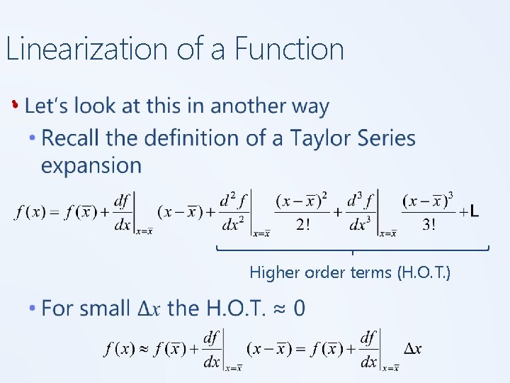
Linearization of a Function • Higher order terms (H. O. T. )

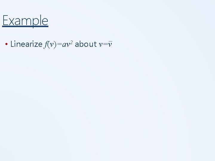
Example _ • Linearize f(v)=av 2 about v=v

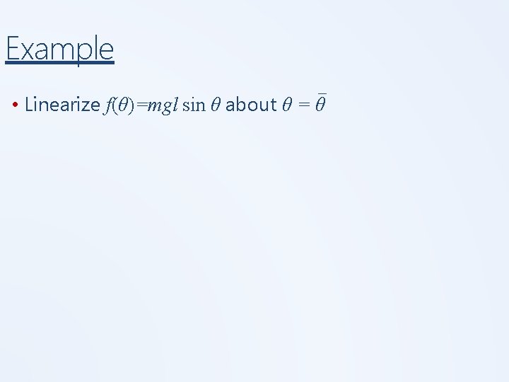
Example _ • Linearize f(θ)=mgl sin θ about θ = θ

Nonlinear Systems • This same idea can be used for providing approximate models of nonlinear systems • Nonlinear diff eq Linear diff eq in terms of deviation from the operating point (Δ) • These approximate models are only valid in a small neighborhood about the operating point

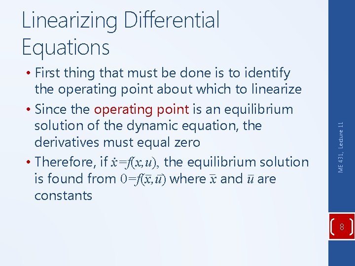
• First thing that must be done is to identify the operating point about which to linearize • Since the operating point is an equilibrium solution of the dynamic equation, the derivatives must equal zero. • Therefore, if x=f(x, u), the equilibrium solution _ _ is found from 0=f(x, u) where x and u are constants ME 431, Lecture 11 Linearizing Differential Equations 8

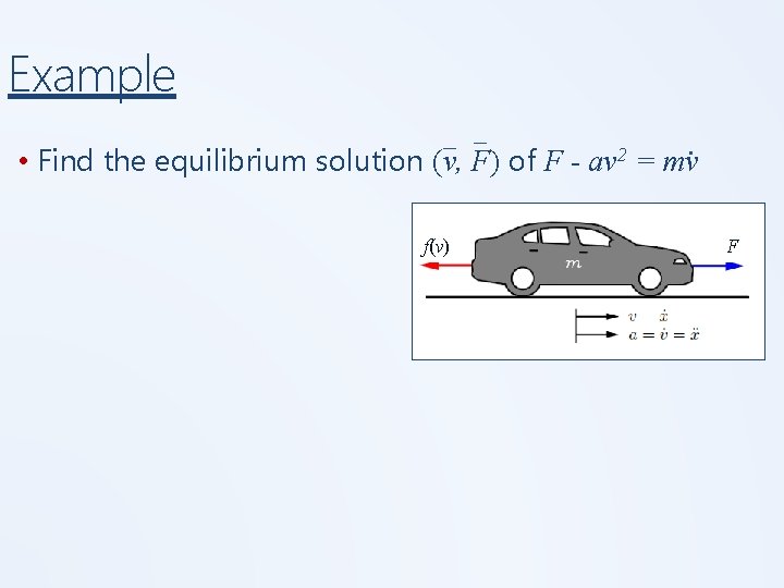
Example _ _ • Find the equilibrium solution (v, F) of F f(v) av 2 . = mv F

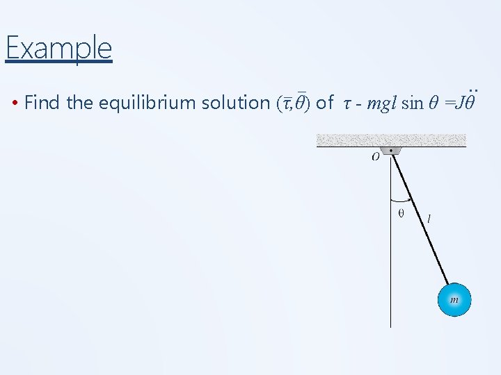
Example __ . . • Find the equilibrium solution (τ, θ) of τ - mgl sin θ =Jθ

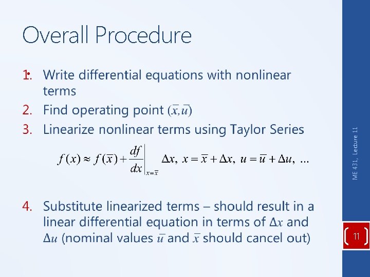
Overall Procedure • ME 431, Lecture 11 __ _ _ 11

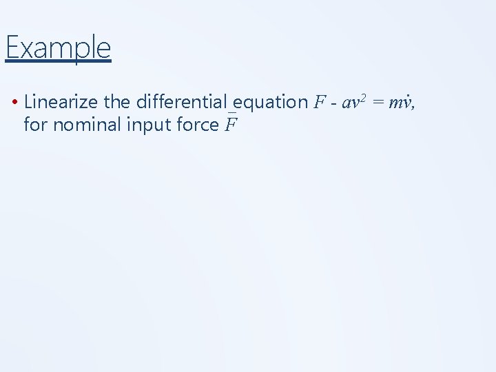
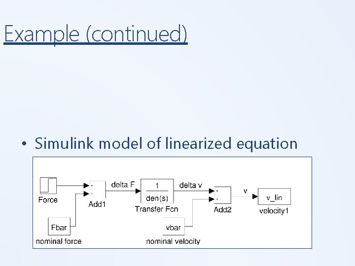
Example • Linearize the differential_equation F for nominal input force F av 2 . = mv,

Example (continued) • Simulink model of linearized equation

Example. . • Linearize the differential equation τ - mgl sin θ =Jθ, _ for nominal input torque τ

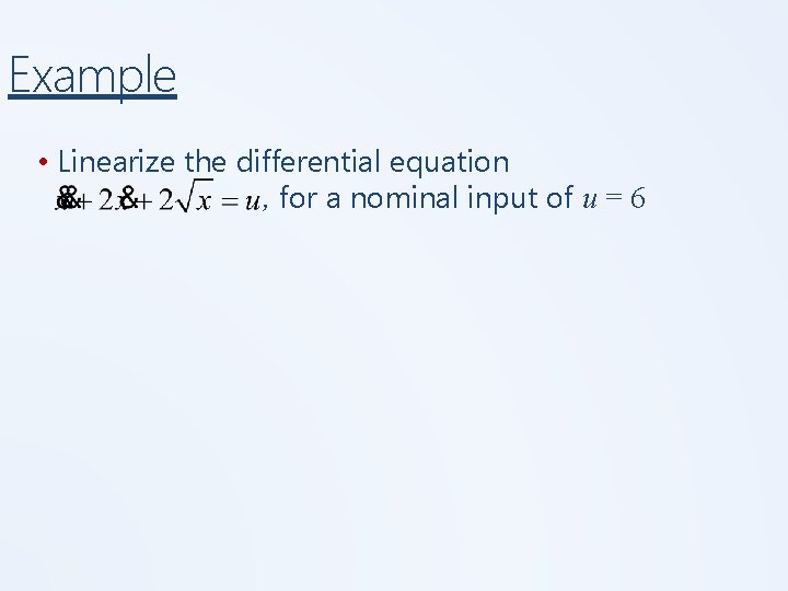
Example • Linearize the differential equation , for a nominal input of u = 6

Example (continued)