Differentials A quick Review on Linear Approximations and


 = 1 + sin x at")


 If f(3) =8, f’(3) = -4, then find f(3. 02)")
 ≈ f(a) + f’(a)(x – a) L(x) = f(a) + f’(a)(x –")


. Now consider a generic value")

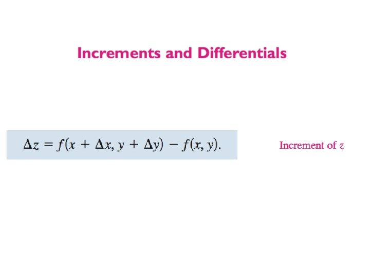
 z By subtracting the z-coordinates: Since the y-coordinate is constant,")


- Slides: 31
Differentials
A quick Review on Linear Approximations and Differentials of a function of one Variable
Key Points: n Understand the concept of a tangent line approximation/linear approx. . n Compare the value of the differential, dy, with the actual change in y, Δy. n Find the differential of a function using differentiation formulas.
Tangent Line Approximation • Consider a tangent to a function at a point x = a y=f(x) • The equation of the tangent line: f(a) • y = f(a) + f ‘(a)(x – a) a • Close to the point, the tangent line is an approximation for f(x)
Start with the point/slope equation: linearization of is the standard linear approximation of f at a.
Example-1: Find the tangent line approximation of f(x) = 1 + sin x at the point (0, 1). Then use a table to compare the y-values of the linear function with those of f(x) on an open interval containing x = 0.
The table compares the values of y given by this linear approximation with the values of f(x) near x = 0. Notice that the closer x is to 0, the better the approximation is.
This conclusion is reinforced by the graph shown in
Example-2: Determine the linear approximation for at a=8. Use the linear approximation to compute
Differentials: When we first started to talk about derivatives, we said that becomes when the change in x and change in y very small. dy can be considered a very small change in y. dx can be considered a very small change in x. become
Now Look at dy • x • y • x + x x = dx • dy = rise of tangent relative to x = dx • y = change in y that occurs relative to x = dx
The Figure below shows the geometric comparison of dy and Δy.
Animated Graphical View • Note how the Δy and the dy in the figure get closer and closer
Let The differential be a differentiable function. is an independent variable. is: is called the differential of y * It is an approximation of the actual change of y for a small change of x
Example-3: Find the differential of Y = 3 – 2 5 x
Example 4: Comparing Δy and dy Let y = x 2. Find dy when x = 1 and dx = 0. 01. Compare this value with Δy for x = 1 and Δx = 0. 01. Solution: Because y = f(x) = x 2, you have f'(x) = 2 x, and the differential dy is given by dy = f'(x)dx = f'(1)(0. 01) = 2(0. 01) = 0. 02. Now, using Δx = 0. 01, the change in y is Δy = f(x + Δx) – f(x) = f(1. 01) – f(1) = (1. 01)2 – 12 = 0. 0201.
Try Me: Linearization (Estimation) If f(3) =8, f’(3) = -4, then find f(3. 02)
Summary f(x) ≈ f(a) + f’(a)(x – a) L(x) = f(a) + f’(a)(x – a) ∆y = f(x + ∆x) – f(x) dx = ∆x dy = f’(x)dx ∆ y≈ dy Differential represents a change in the linearization of a function.
Can you extend this concept to functions of two and more variables?
Definition of Total Differential
Re-Review on Function of one variable: y = f(x). Now consider a generic value of x with a tangent to the curve at (x, f(x)). Compare the initial value of x to a value of x that is slightly larger. The slope of the tangent line is: Since and since dx is being defined as “run” then dy becomes “rise” by definition. For small values of dx, the rise of the tangent line, was used as an approximation for delta y , the change in the function.
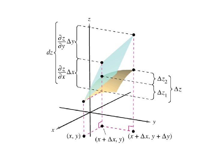
Now let’s extend this concept to functions of several variables. Consider an input (x, y) for this function. Its outputs z = f(x, y) create a set of points (x, y, z) that form the surface you see below. The differential dz will have two parts: one part generated by a change in x and the other part generated by a change in y. z z = f(x, y) Consider a new point in the domain generated by a small change in x. Now consider the functional image of the new point. We can use the function to calculate , the difference between the two z-coordinates. By subtracting the z-coordinates: x y
z = f(x, y) z By subtracting the z-coordinates: Since the y-coordinate is constant, we can use that cross section to draw the tangent to Remember that, dz is the change in the height of the tangent line, and can be used to estimate the change in z. dz x y
Since there has been no change in y we can express the differential so far in terms of the change in x: Now track the influence on z when a new point is generated by a change in the y direction. z = f(x, y) z Now that the change in z is generated by changes in x and y, we can define the total differential: x y
Class work Compute the total differential
Example 7. A right circular cylinder has a height of 5 ft. and a radius of 2 ft. These measurements have possible errors in accuracy as laid out in the table below. Complete the table below. Comment on the relationship between d. V and for the indicated errors. 0. 1 ft. 7. 54 cu ft 0. 01 ft. . 754 cu ft 0. 001 ft. . 075 cu ft
0. 1 ft. 7. 54 cu ft 7. 826 cu ft 0. 01 ft. . 754 cu ft 0. 757 cu ft . 075 cu ft 0. 001 ft.
Try Me Find the total differential of