7 1 LINEAR AND NONLINEAR SYSTEMS OF EQUATIONS

7. 1 LINEAR AND NONLINEAR SYSTEMS OF EQUATIONS Copyright © Cengage Learning. All rights reserved.

What You Should Learn • Use the method of substitution to solve systems of linear equations in two variables. • Use the method of substitution to solve systems of nonlinear equations in two variables. • Use a graphical approach to solve systems of equations in two variables. • Use systems of equations to model and solve real-life problems. 2

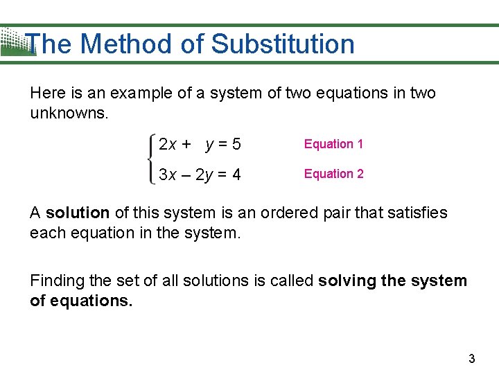
The Method of Substitution Here is an example of a system of two equations in two unknowns. 2 x + y = 5 Equation 1 3 x – 2 y = 4 Equation 2 A solution of this system is an ordered pair that satisfies each equation in the system. Finding the set of all solutions is called solving the system of equations. 3

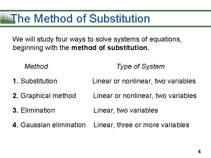
The Method of Substitution We will study four ways to solve systems of equations, beginning with the method of substitution. Method Type of System 1. Substitution Linear or nonlinear, two variables 2. Graphical method Linear or nonlinear, two variables 3. Elimination Linear, two variables 4. Gaussian elimination Linear, three or more variables 4

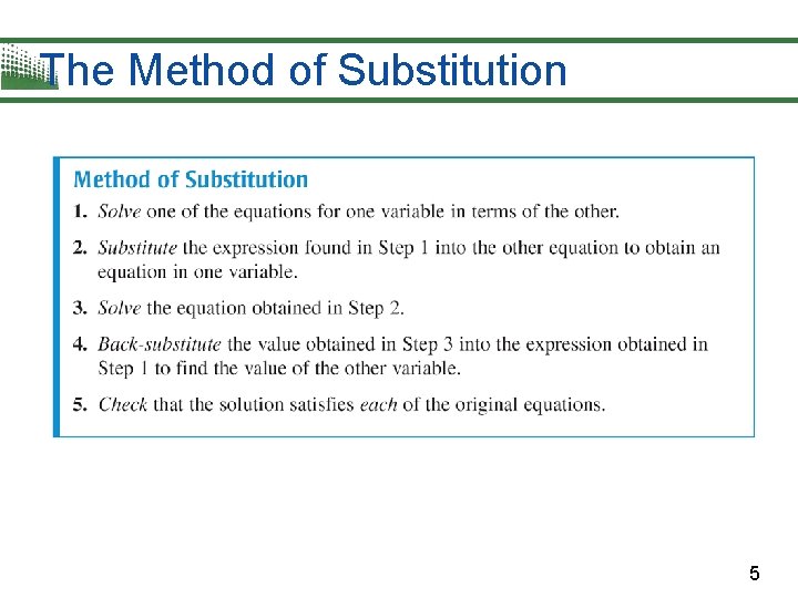
The Method of Substitution 5

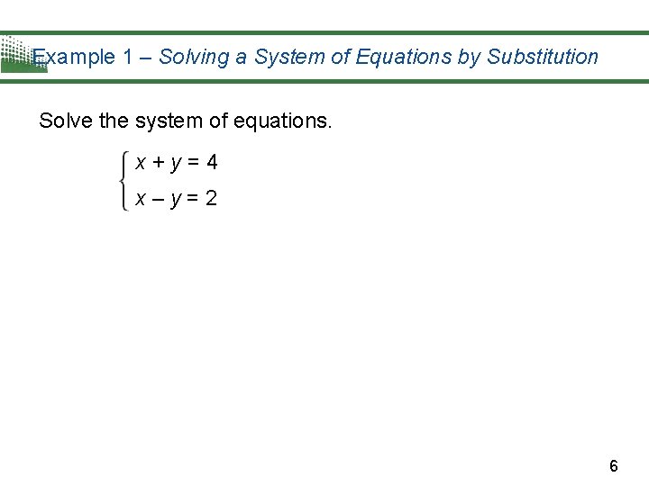
Example 1 – Solving a System of Equations by Substitution Solve the system of equations. x+y=4 x–y=2 6

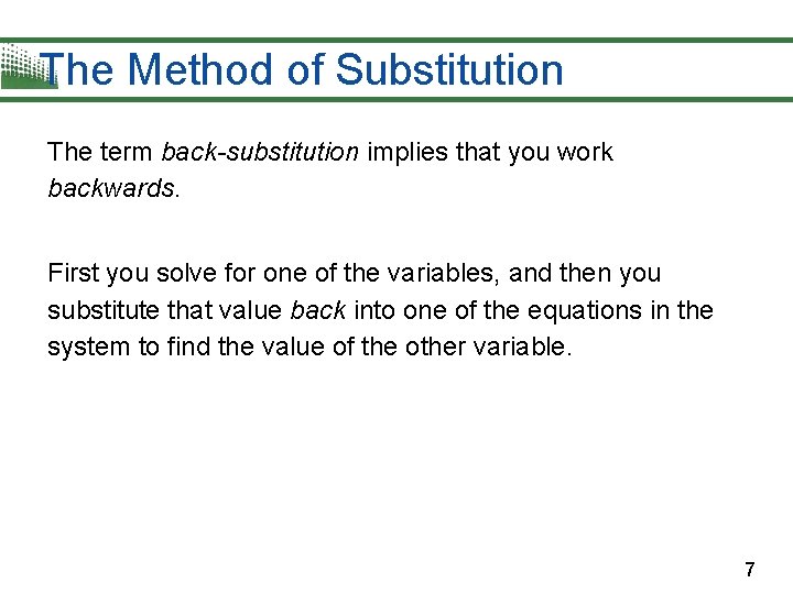
The Method of Substitution The term back-substitution implies that you work backwards. First you solve for one of the variables, and then you substitute that value back into one of the equations in the system to find the value of the other variable. 7

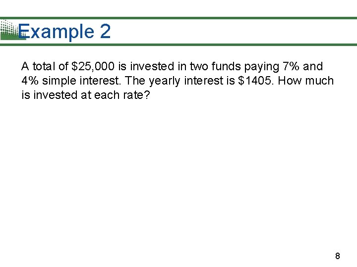
Example 2 A total of $25, 000 is invested in two funds paying 7% and 4% simple interest. The yearly interest is $1405. How much is invested at each rate? 8

Nonlinear Systems of Equations The equations in Example 1 and 2 are linear. The method of substitution can also be used to solve systems in which one or both of the equations are nonlinear. 9

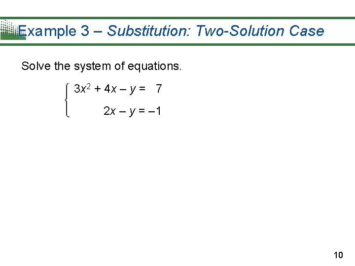
Example 3 – Substitution: Two-Solution Case Solve the system of equations. 3 x 2 + 4 x – y = 7 2 x – y = – 1 10

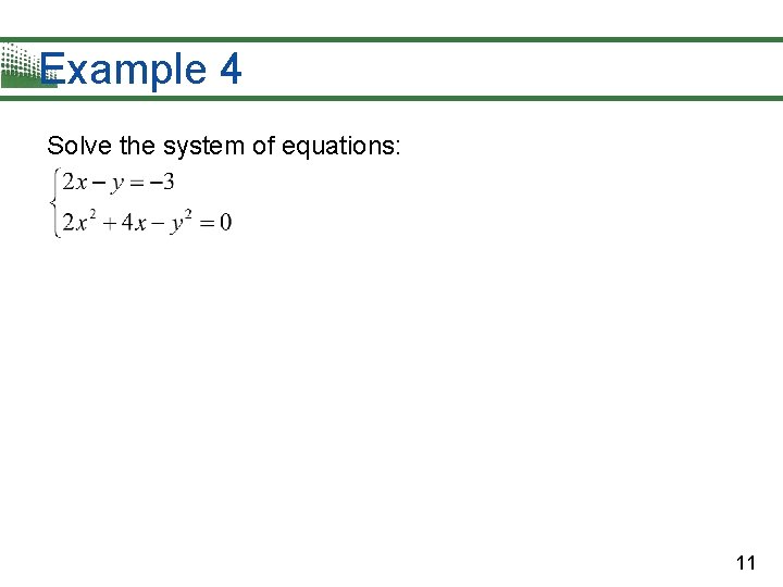
Example 4 Solve the system of equations: 11

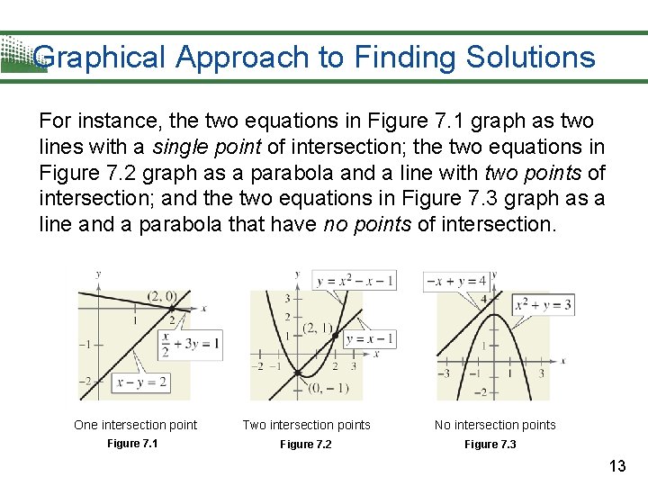
Graphical Approach to Finding Solutions From Example 3, we can see that a system of two equations in two unknowns can have exactly one solution, more than one solution, or no solution. By using a graphical method, you can gain insight about the number of solutions and the location(s) of the solution(s) of a system of equations by graphing each of the equations in the same coordinate plane. The solutions of the system correspond to the points of intersection of the graphs. 12

Graphical Approach to Finding Solutions For instance, the two equations in Figure 7. 1 graph as two lines with a single point of intersection; the two equations in Figure 7. 2 graph as a parabola and a line with two points of intersection; and the two equations in Figure 7. 3 graph as a line and a parabola that have no points of intersection. One intersection point Two intersection points Figure 7. 1 Figure 7. 2 No intersection points Figure 7. 3 13

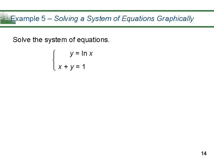
Example 5 – Solving a System of Equations Graphically Solve the system of equations. y = ln x x+y=1 14

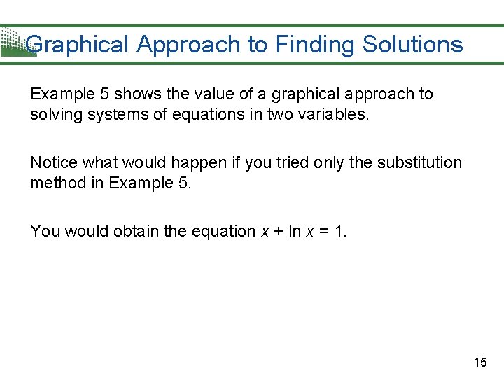
Graphical Approach to Finding Solutions Example 5 shows the value of a graphical approach to solving systems of equations in two variables. Notice what would happen if you tried only the substitution method in Example 5. You would obtain the equation x + ln x = 1. 15

Applications The total cost C of producing x units of a product typically has two components—the initial cost and the cost per unit. When enough units have been sold so that the total revenue R equals the total cost C, the sales are said to have reached the break-even point. You will find that the break-even point corresponds to the point of intersection of the cost and revenue curves. 16

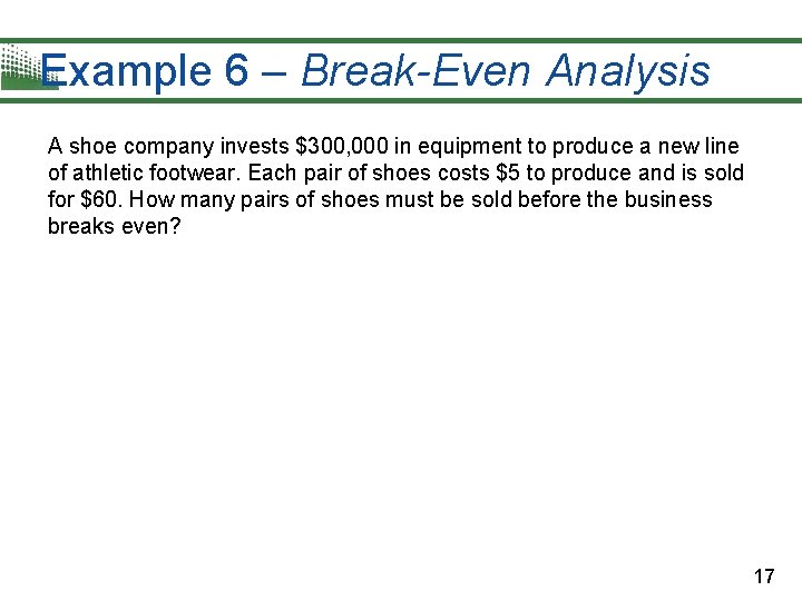
Example 6 – Break-Even Analysis A shoe company invests $300, 000 in equipment to produce a new line of athletic footwear. Each pair of shoes costs $5 to produce and is sold for $60. How many pairs of shoes must be sold before the business breaks even? 17

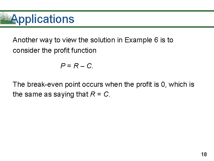
Applications Another way to view the solution in Example 6 is to consider the profit function P = R – C. The break-even point occurs when the profit is 0, which is the same as saying that R = C. 18

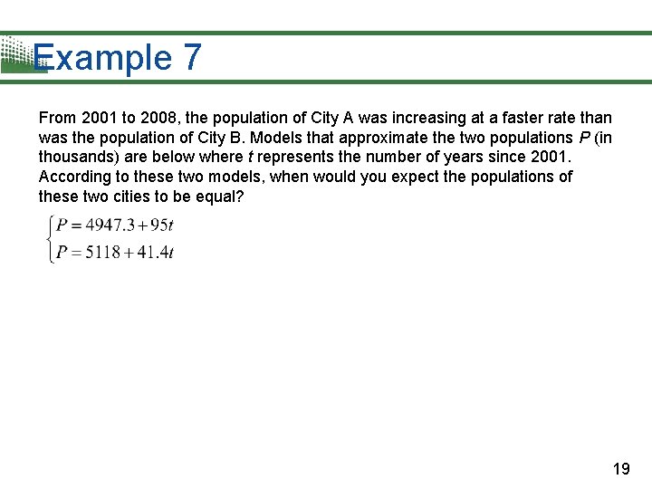
Example 7 From 2001 to 2008, the population of City A was increasing at a faster rate than was the population of City B. Models that approximate the two populations P (in thousands) are below where t represents the number of years since 2001. According to these two models, when would you expect the populations of these two cities to be equal? 19