KS 4 Mathematics D 2 Averages and range

KS 4 Mathematics D 2 Averages and range 1 of 49 © Boardworks Ltd 2005

Contents D 2 Averages and range A D 2. 1 The mode A D 2. 2 The mean A D 2. 3 Calculating the mean from frequency tables A D 2. 4 The median A D 2. 5 Comparing data 2 of 49 © Boardworks Ltd 2005

The three averages and range There are three different types of average: MODE MEAN MEDIAN most common sum of values number of values middle value The range is not an average, but tells you how the data is spread out: RANGE largest value – smallest value 3 of 49 © Boardworks Ltd 2005

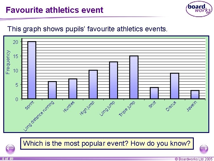
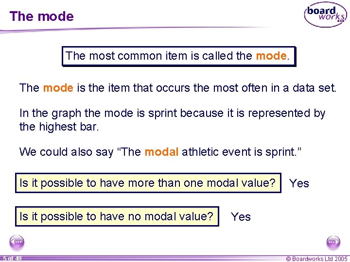
Favourite athletics event This graph shows pupils’ favourite athletics events. Frequency 20 15 10 5 in Ja ve l Sh ot is cu s D Tr ip le ju m p p ju m g Lo n m p ju ig h H ur dl es H Lo n g di s ta nc e ru nn Sp rin t in g 0 Which is the most popular event? How do you know? 4 of 49 © Boardworks Ltd 2005

The mode The most common item is called the mode. The mode is the item that occurs the most often in a data set. In the graph the mode is sprint because it is represented by the highest bar. We could also say “The modal athletic event is sprint. ” Is it possible to have more than one modal value? Is it possible to have no modal value? 5 of 49 Yes © Boardworks Ltd 2005

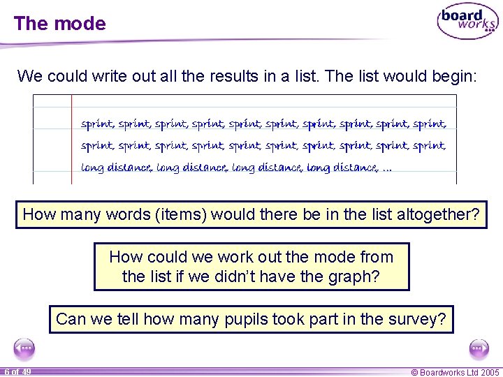
The mode We could write out all the results in a list. The list would begin: How many words (items) would there be in the list altogether? How could we work out the mode from the list if we didn’t have the graph? Can we tell how many pupils took part in the survey? 6 of 49 © Boardworks Ltd 2005

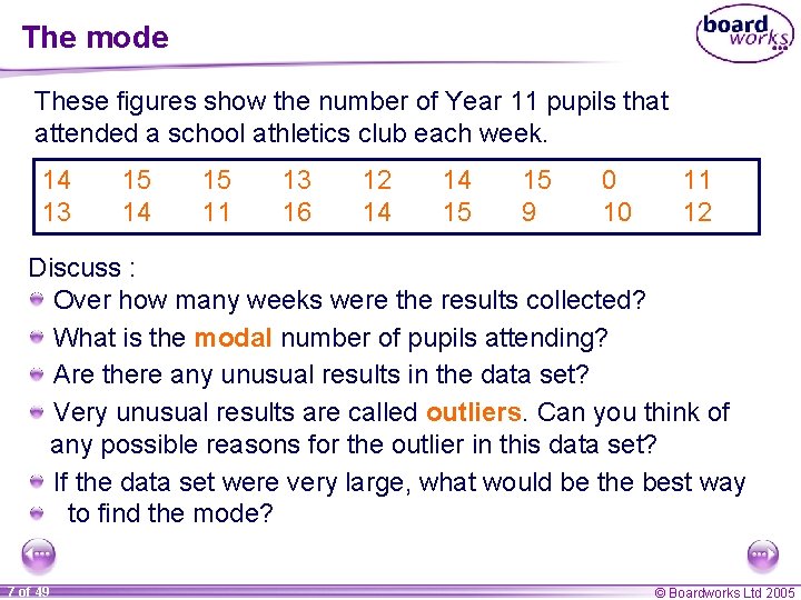
The mode These figures show the number of Year 11 pupils that attended a school athletics club each week. 14 13 15 14 15 11 13 16 12 14 14 15 15 9 0 10 11 12 Discuss : Over how many weeks were the results collected? What is the modal number of pupils attending? Are there any unusual results in the data set? Very unusual results are called outliers. Can you think of any possible reasons for the outlier in this data set? If the data set were very large, what would be the best way to find the mode? 7 of 49 © Boardworks Ltd 2005

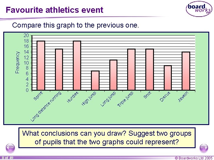
Favourite athletics event in Ja ve l Sh ot is cu s D Tr ip le ju m p p ju m g Lo n m p ju ig h H ur dl es H Lo n g di st an ce ru nn in g 20 18 16 14 12 10 8 6 4 2 0 Sp rin t Frequency Compare this graph to the previous one. What conclusions can you draw? Suggest two groups of pupils that the two graphs could represent? 8 of 49 © Boardworks Ltd 2005

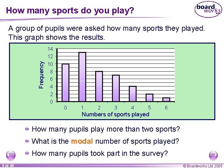
How many sports do you play? A group of pupils were asked how many sports they played. This graph shows the results. Frequency 14 12 10 8 6 4 2 0 0 1 2 3 4 5 6 Numbers of sports played How many pupils play more than two sports? What is the modal number of sports played? How many pupils took part in the survey? 9 of 49 © Boardworks Ltd 2005

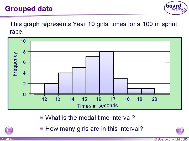
Grouped data This graph represents Year 10 girls’ times for a 100 m sprint race. Frequency 10 8 6 4 2 0 12 13 14 15 16 17 18 19 20 Times in seconds What is the modal time interval? How many girls are in this interval? 10 of 49 © Boardworks Ltd 2005

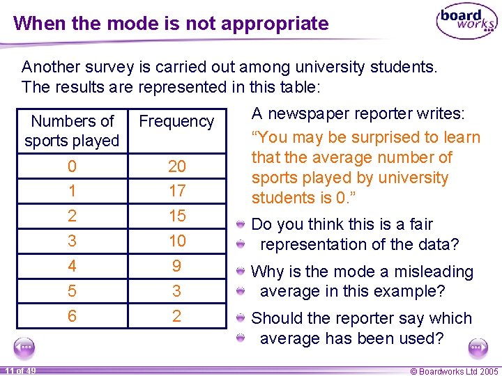
When the mode is not appropriate Another survey is carried out among university students. The results are represented in this table: Numbers of sports played Frequency 0 20 1 17 2 15 3 10 4 9 5 3 6 2 11 of 49 A newspaper reporter writes: “You may be surprised to learn that the average number of sports played by university students is 0. ” Do you think this is a fair representation of the data? Why is the mode a misleading average in this example? Should the reporter say which average has been used? © Boardworks Ltd 2005

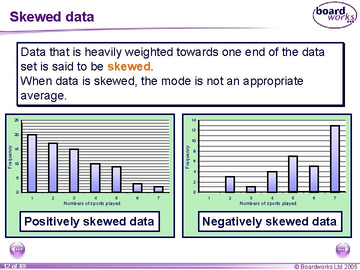
Skewed data Data that is heavily weighted towards one end of the data set is said to be skewed. When data is skewed, the mode is not an appropriate average. 25 14 12 20 Frequency 10 15 10 8 6 4 5 2 0 0 1 2 3 4 5 6 Numbers of sports played Positively skewed data 12 of 49 7 1 2 3 4 5 6 7 Numbers of sports played Negatively skewed data © Boardworks Ltd 2005

Contents D 2 Averages and range A D 2. 1 The mode A D 2. 2 The mean A D 2. 3 Calculating the mean from frequency tables A D 2. 4 The median A D 2. 5 Comparing data 13 of 49 © Boardworks Ltd 2005

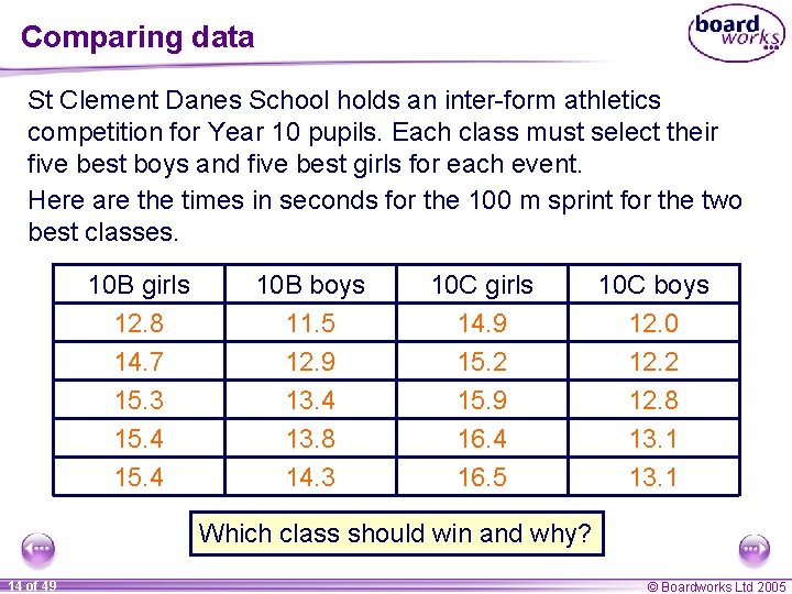
Comparing data St Clement Danes School holds an inter-form athletics competition for Year 10 pupils. Each class must select their five best boys and five best girls for each event. Here are the times in seconds for the 100 m sprint for the two best classes. 10 B girls 12. 8 14. 7 15. 3 15. 4 10 B boys 11. 5 12. 9 13. 4 13. 8 14. 3 10 C girls 14. 9 15. 2 15. 9 16. 4 16. 5 10 C boys 12. 0 12. 2 12. 8 13. 1 Which class should win and why? 14 of 49 © Boardworks Ltd 2005

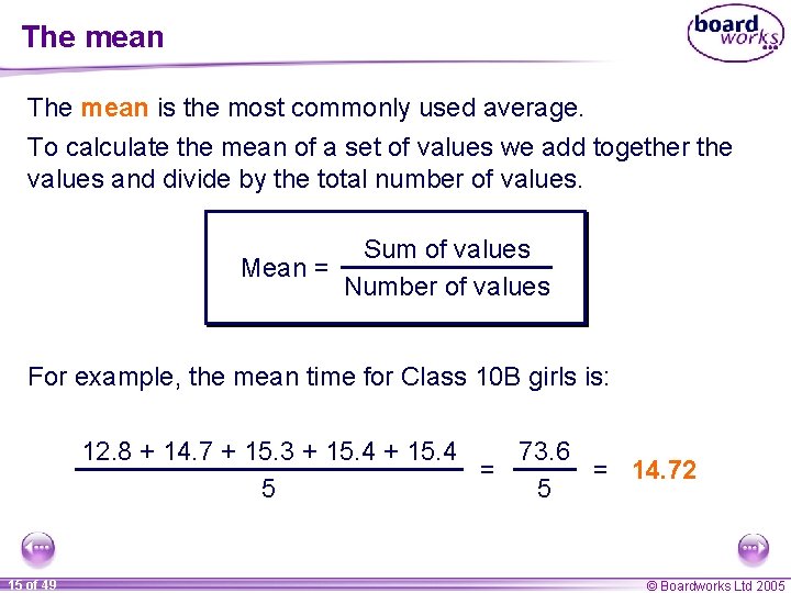
The mean is the most commonly used average. To calculate the mean of a set of values we add together the values and divide by the total number of values. Sum of values Mean = Number of values For example, the mean time for Class 10 B girls is: 12. 8 + 14. 7 + 15. 3 + 15. 4 73. 6 = = 14. 72 5 5 15 of 49 © Boardworks Ltd 2005

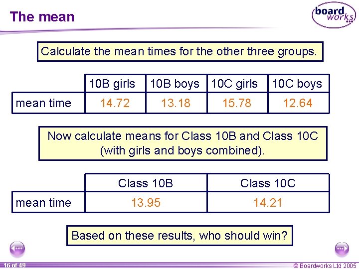
The mean Calculate the mean times for the other three groups. 10 B girls mean time 10 B boys 10 C girls 14. 72 13. 18 15. 78 10 C boys 12. 64 Now calculate means for Class 10 B and Class 10 C (with girls and boys combined). mean time Class 10 B Class 10 C 13. 95 14. 21 Based on these results, who should win? 16 of 49 © Boardworks Ltd 2005

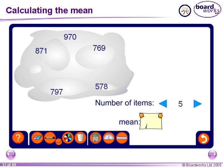
Calculating the mean 17 of 49 © Boardworks Ltd 2005

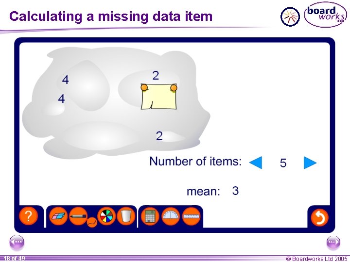
Calculating a missing data item 18 of 49 © Boardworks Ltd 2005

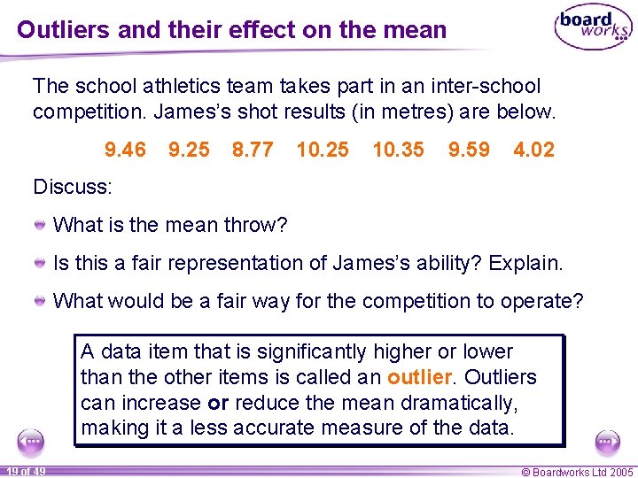
Outliers and their effect on the mean The school athletics team takes part in an inter-school competition. James’s shot results (in metres) are below. 9. 46 9. 25 8. 77 10. 25 10. 35 9. 59 4. 02 Discuss: What is the mean throw? Is this a fair representation of James’s ability? Explain. What would be a fair way for the competition to operate? A data item that is significantly higher or lower than the other items is called an outlier. Outliers can increase or reduce the mean dramatically, making it a less accurate measure of the data. 19 of 49 © Boardworks Ltd 2005

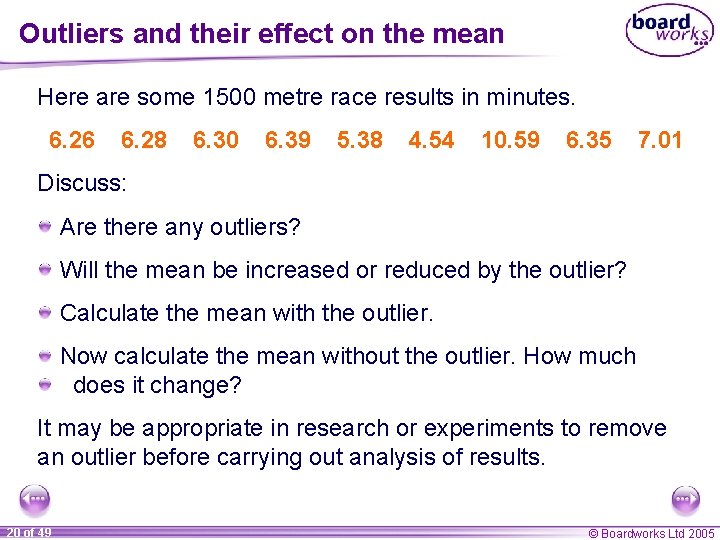
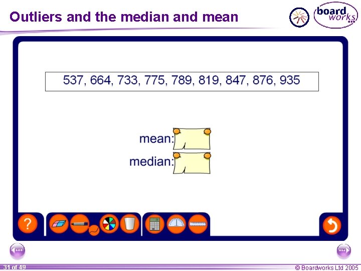
Outliers and their effect on the mean Here are some 1500 metre race results in minutes. 6. 26 6. 28 6. 30 6. 39 5. 38 4. 54 10. 59 6. 35 7. 01 Discuss: Are there any outliers? Will the mean be increased or reduced by the outlier? Calculate the mean with the outlier. Now calculate the mean without the outlier. How much does it change? It may be appropriate in research or experiments to remove an outlier before carrying out analysis of results. 20 of 49 © Boardworks Ltd 2005

Contents D 2 Averages and range A D 2. 1 The mode A D 2. 2 The mean A D 2. 3 Calculating the mean from frequency tables A D 2. 4 The median A D 2. 5 Comparing data 21 of 49 © Boardworks Ltd 2005

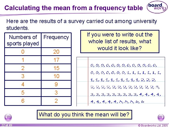
Calculating the mean from a frequency table Here are the results of a survey carried out among university students. If you were to write out the Numbers of Frequency whole list of results, what sports played would it look like? 0 20 1 17 2 15 3 10 4 9 5 3 6 2 What do you think the mean will be? 22 of 49 © Boardworks Ltd 2005

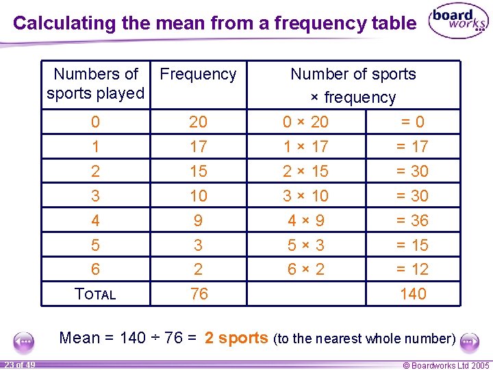
Calculating the mean from a frequency table Numbers of Frequency sports played 0 1 2 3 4 5 6 TOTAL 20 17 15 10 9 3 2 76 Number of sports × frequency 0 × 20 1 × 17 2 × 15 3 × 10 4× 9 5× 3 6× 2 =0 = 17 = 30 = 36 = 15 = 12 140 Mean = 140 ÷ 76 = 2 sports (to the nearest whole number) 23 of 49 © Boardworks Ltd 2005

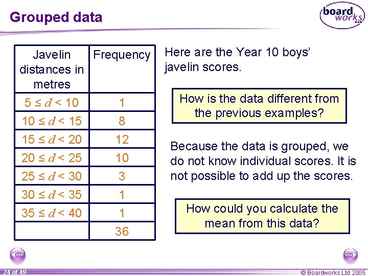
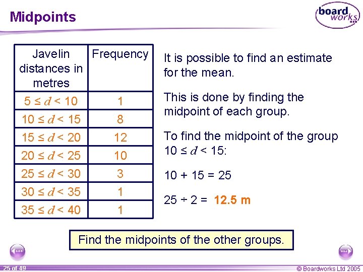
Grouped data Javelin Frequency distances in metres 5 ≤ d < 10 1 10 ≤ d < 15 8 15 ≤ d < 20 20 ≤ d < 25 25 ≤ d < 30 30 ≤ d < 35 35 ≤ d < 40 24 of 49 12 10 3 1 1 36 Here are the Year 10 boys’ javelin scores. How is the data different from the previous examples? Because the data is grouped, we do not know individual scores. It is not possible to add up the scores. How could you calculate the mean from this data? © Boardworks Ltd 2005

Midpoints Javelin Frequency distances in metres 5 ≤ d < 10 1 10 ≤ d < 15 8 It is possible to find an estimate for the mean. 15 ≤ d < 20 20 ≤ d < 25 25 ≤ d < 30 30 ≤ d < 35 35 ≤ d < 40 To find the midpoint of the group 10 ≤ d < 15: 12 10 3 1 1 This is done by finding the midpoint of each group. 10 + 15 = 25 25 ÷ 2 = 12. 5 m Find the midpoints of the other groups. 25 of 49 © Boardworks Ltd 2005

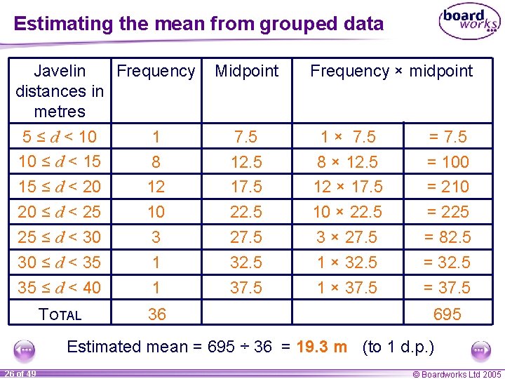
Estimating the mean from grouped data Javelin Frequency distances in metres 5 ≤ d < 10 1 10 ≤ d < 15 8 15 ≤ d < 20 12 20 ≤ d < 25 10 25 ≤ d < 30 3 30 ≤ d < 35 1 35 ≤ d < 40 1 TOTAL 36 Midpoint 7. 5 12. 5 17. 5 22. 5 27. 5 32. 5 37. 5 Frequency × midpoint 1 × 7. 5 8 × 12. 5 12 × 17. 5 10 × 22. 5 3 × 27. 5 1 × 32. 5 1 × 37. 5 = 100 = 210 = 225 = 82. 5 = 37. 5 695 Estimated mean = 695 ÷ 36 = 19. 3 m (to 1 d. p. ) 26 of 49 © Boardworks Ltd 2005

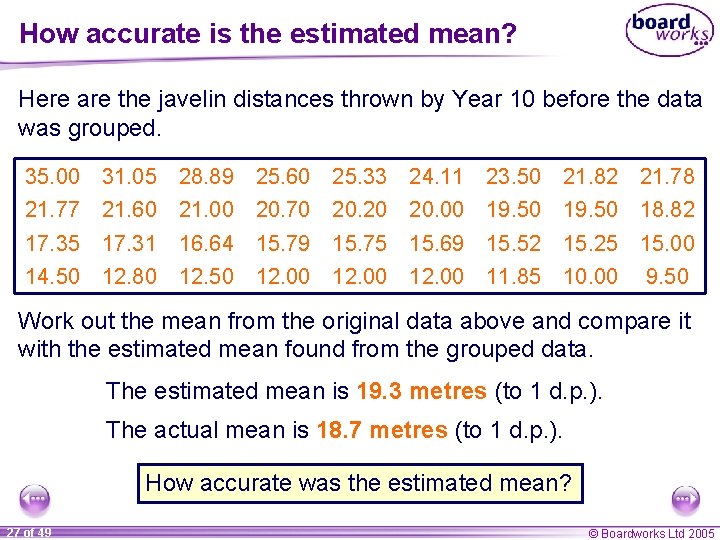
How accurate is the estimated mean? Here are the javelin distances thrown by Year 10 before the data was grouped. 35. 00 31. 05 28. 89 25. 60 25. 33 24. 11 23. 50 21. 82 21. 78 21. 77 21. 60 21. 00 20. 70 20. 20 20. 00 19. 50 18. 82 17. 35 17. 31 16. 64 15. 79 15. 75 15. 69 15. 52 15. 25 15. 00 14. 50 12. 80 12. 50 12. 00 11. 85 10. 00 9. 50 Work out the mean from the original data above and compare it with the estimated mean found from the grouped data. The estimated mean is 19. 3 metres (to 1 d. p. ). The actual mean is 18. 7 metres (to 1 d. p. ). How accurate was the estimated mean? 27 of 49 © Boardworks Ltd 2005

Contents D 2 Averages and range A D 2. 1 The mode A D 2. 2 The mean A D 2. 3 Calculating the mean from frequency tables A D 2. 4 The median A D 2. 5 Comparing data 28 of 49 © Boardworks Ltd 2005

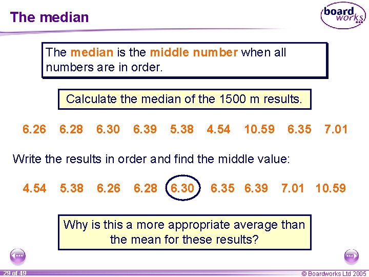
The median is the middle number when all numbers are in order. Calculate the median of the 1500 m results. 6. 26 6. 28 6. 30 6. 39 5. 38 4. 54 10. 59 6. 35 7. 01 Write the results in order and find the middle value: 4. 54 5. 38 6. 26 6. 28 6. 30 6. 35 6. 39 7. 01 10. 59 Why is this a more appropriate average than the mean for these results? 29 of 49 © Boardworks Ltd 2005

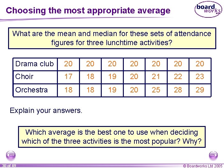
Choosing the most appropriate average What are the mean and median for these sets of attendance figures for three lunchtime activities? Drama club 20 20 Choir 17 18 19 20 21 22 23 Orchestra 18 18 19 20 25 28 29 Explain your answers. Which average is the best one to use when deciding which of the three activities is the most popular? Why? 30 of 49 © Boardworks Ltd 2005

Outliers and the median and mean 31 of 49 © Boardworks Ltd 2005

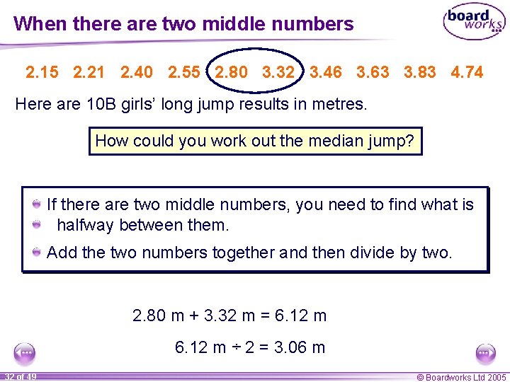
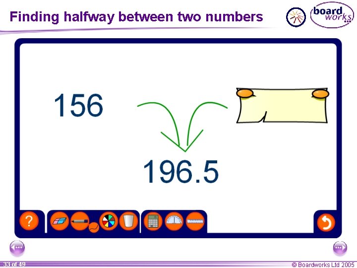
When there are two middle numbers 2. 15 2. 21 2. 40 2. 55 2. 80 3. 32 3. 46 3. 63 3. 83 4. 74 Here are 10 B girls’ long jump results in metres. How could you work out the median jump? If there are two middle numbers, you need to find what is halfway between them. Add the two numbers together and then divide by two. 2. 80 m + 3. 32 m = 6. 12 m ÷ 2 = 3. 06 m 32 of 49 © Boardworks Ltd 2005

Finding halfway between two numbers 33 of 49 © Boardworks Ltd 2005

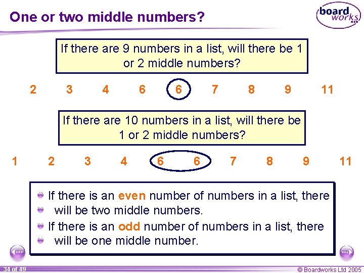
One or two middle numbers? If there are 9 numbers in a list, will there be 1 or 2 middle numbers? 2 3 4 6 6 7 8 9 11 If there are 10 numbers in a list, will there be 1 or 2 middle numbers? 1 2 3 4 6 6 7 8 9 11 If there is an even number of numbers in a list, there will be two middle numbers. If there is an odd number of numbers in a list, there will be one middle number. 34 of 49 © Boardworks Ltd 2005

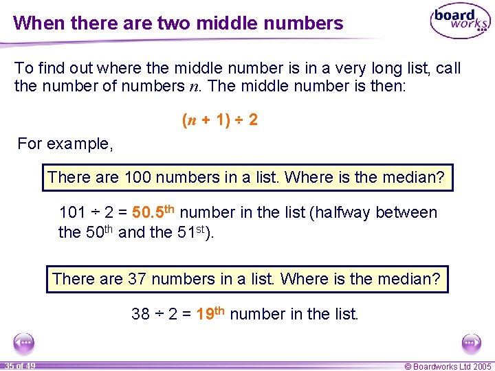
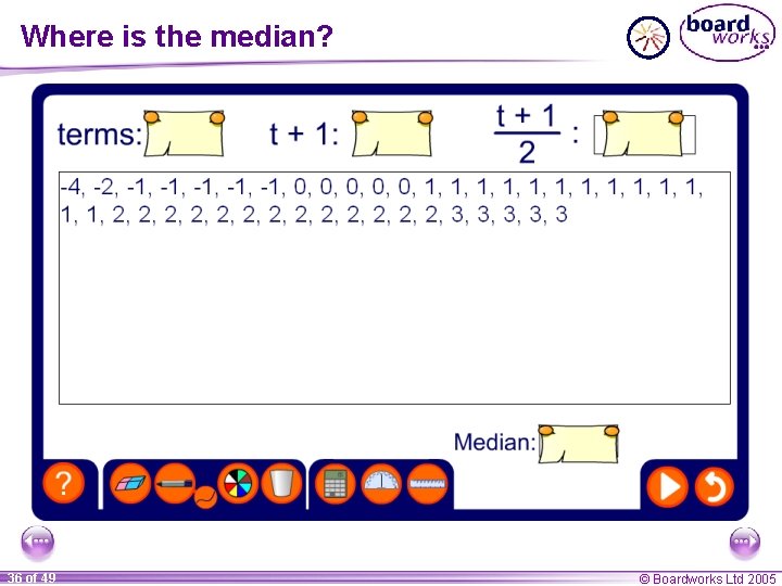
When there are two middle numbers To find out where the middle number is in a very long list, call the number of numbers n. The middle number is then: (n + 1) ÷ 2 For example, There are 100 numbers in a list. Where is the median? 101 ÷ 2 = 50. 5 th number in the list (halfway between the 50 th and the 51 st). There are 37 numbers in a list. Where is the median? 38 ÷ 2 = 19 th number in the list. 35 of 49 © Boardworks Ltd 2005

Where is the median? 36 of 49 © Boardworks Ltd 2005

Contents D 2 Averages and range A D 2. 1 The mode A D 2. 2 The mean A D 2. 3 Calculating the mean from frequency tables A D 2. 4 The median A D 2. 5 Comparing data 37 of 49 © Boardworks Ltd 2005

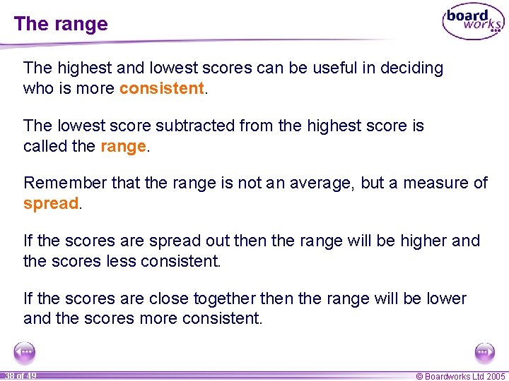
The range The highest and lowest scores can be useful in deciding who is more consistent. The lowest score subtracted from the highest score is called the range. Remember that the range is not an average, but a measure of spread. If the scores are spread out then the range will be higher and the scores less consistent. If the scores are close together then the range will be lower and the scores more consistent. 38 of 49 © Boardworks Ltd 2005

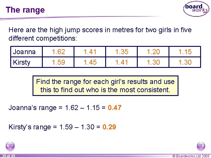
The range Here are the high jump scores in metres for two girls in five different competitions: Joanna Kirsty 1. 62 1. 59 1. 41 1. 45 1. 35 1. 41 1. 20 1. 30 1. 15 1. 30 Find the range for each girl’s results and use this to find out who is the most consistent. Joanna’s range = 1. 62 – 1. 15 = 0. 47 Kirsty’s range = 1. 59 – 1. 30 = 0. 29 39 of 49 © Boardworks Ltd 2005

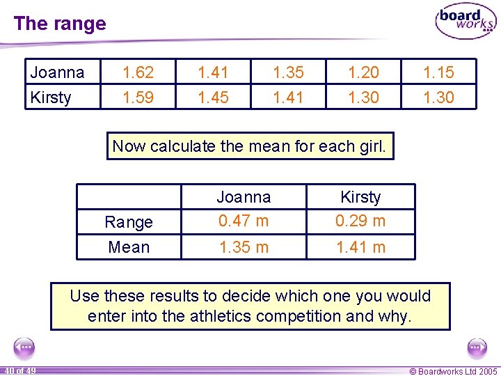
The range Joanna Kirsty 1. 62 1. 59 1. 41 1. 45 1. 35 1. 41 1. 20 1. 30 1. 15 1. 30 Now calculate the mean for each girl. Range Mean Joanna 0. 47 m Kirsty 0. 29 m 1. 35 m 1. 41 m Use these results to decide which one you would enter into the athletics competition and why. 40 of 49 © Boardworks Ltd 2005

Calculating the mean, median and range 41 of 49 © Boardworks Ltd 2005

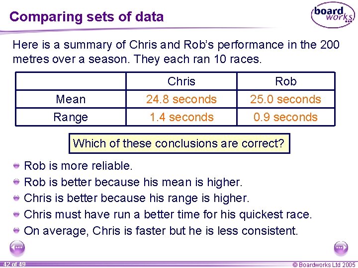
Comparing sets of data Here is a summary of Chris and Rob’s performance in the 200 metres over a season. They each ran 10 races. Mean Range Chris 24. 8 seconds 1. 4 seconds Rob 25. 0 seconds 0. 9 seconds Which of these conclusions are correct? Rob is more reliable. Rob is better because his mean is higher. Chris is better because his range is higher. Chris must have run a better time for his quickest race. On average, Chris is faster but he is less consistent. 42 of 49 © Boardworks Ltd 2005

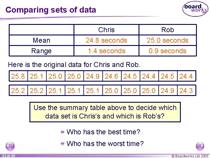
Comparing sets of data Mean Range Chris 24. 8 seconds 1. 4 seconds Rob 25. 0 seconds 0. 9 seconds Here is the original data for Chris and Rob. 25. 8 25. 1 25. 0 24. 9 24. 6 24. 5 24. 4 25. 2 25. 1 25. 0 24. 9 24. 3 Use the summary table above to decide which data set is Chris’s and which is Rob’s? Who has the best time? Who has the worst time? 43 of 49 © Boardworks Ltd 2005

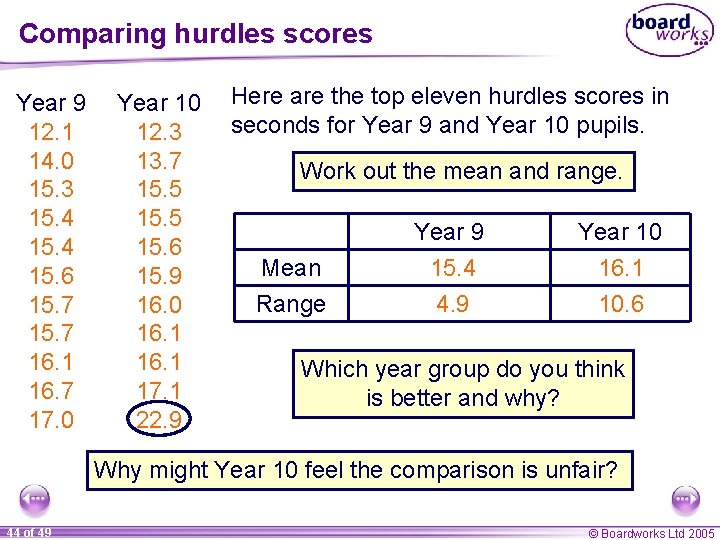
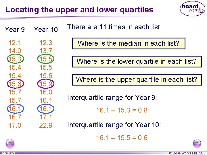
Comparing hurdles scores Year 9 12. 1 14. 0 15. 3 15. 4 15. 6 15. 7 16. 1 16. 7 17. 0 Year 10 12. 3 13. 7 15. 5 15. 6 15. 9 16. 0 16. 1 17. 1 22. 9 Here are the top eleven hurdles scores in seconds for Year 9 and Year 10 pupils. Work out the mean and range. Mean Range Year 9 Year 10 15. 4 4. 9 16. 1 10. 6 Which year group do you think is better and why? Why might Year 10 feel the comparison is unfair? 44 of 49 © Boardworks Ltd 2005

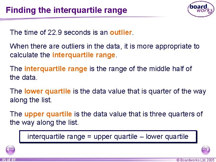
Finding the interquartile range The time of 22. 9 seconds is an outlier. When there are outliers in the data, it is more appropriate to calculate the interquartile range. The interquartile range is the range of the middle half of the data. The lower quartile is the data value that is quarter of the way along the list. The upper quartile is the data value that is three quarters of the way along the list. interquartile range = upper quartile – lower quartile 45 of 49 © Boardworks Ltd 2005

Locating the upper and lower quartiles Year 9 Year 10 12. 1 14. 0 15. 3 15. 4 15. 6 15. 7 16. 1 16. 7 17. 0 12. 3 13. 7 15. 5 15. 6 15. 9 16. 0 16. 1 17. 1 22. 9 There are 11 times in each list. Where is the median in each list? Where is the lower quartile in each list? Where is the upper quartile in each list? Interquartile range for Year 9: 16. 1 – 15. 3 = 0. 8 Interquartile range for Year 10: 16. 1 – 15. 5 = 0. 6 46 of 49 © Boardworks Ltd 2005

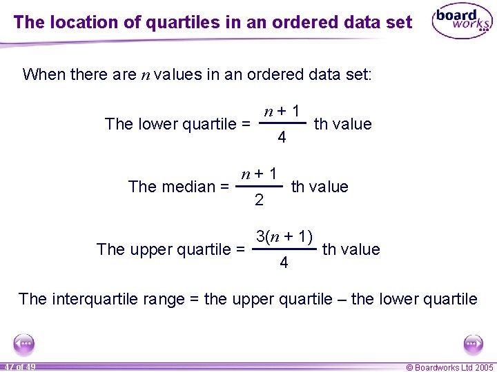
The location of quartiles in an ordered data set When there are n values in an ordered data set: n+1 The lower quartile = The median = 4 n+1 The upper quartile = th value 2 3(n + 1) 4 th value The interquartile range = the upper quartile – the lower quartile 47 of 49 © Boardworks Ltd 2005

Finding the interquartile range 48 of 49 © Boardworks Ltd 2005

Review To review the work you have covered in this topic: 1) Play “Guess the word”. Write out the key words on cards. Shuffle the cards. Describe the word on each card to your partner. Your partner must guess the word. Do as many as you can in one minute, then swap over. 2) Make up challenges involving sets of data for your partner, such as working out the mean. 3) Make a list of possible mistakes to avoid in this topic. 49 of 49 © Boardworks Ltd 2005