Judgment and Decision Making in Information Systems Decision

Judgment and Decision Making in Information Systems Decision Making, Sensitivity Analysis, and the Value of Information Yuval Shahar, M. D. , Ph. D.

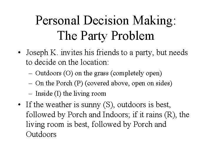
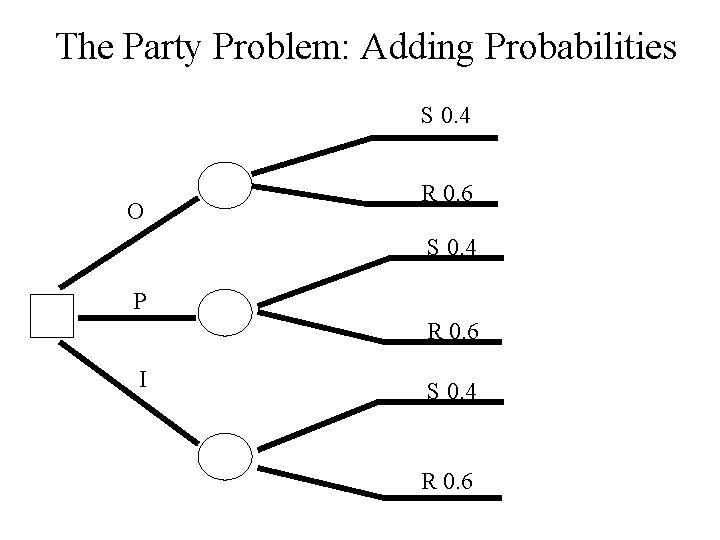
Personal Decision Making: The Party Problem • Joseph K. invites his friends to a party, but needs to decide on the location: – Outdoors (O) on the grass (completely open) – On the Porch (P) (covered above, open on sides) – Inside (I) the living room • If the weather is sunny (S), outdoors is best, followed by Porch and Indoors; if it rains (R), the living room is best, followed by Porch and Outdoors

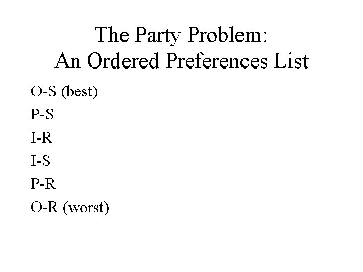
The Party Problem: An Ordered Preferences List O-S (best) P-S I-R I-S P-R O-R (worst)

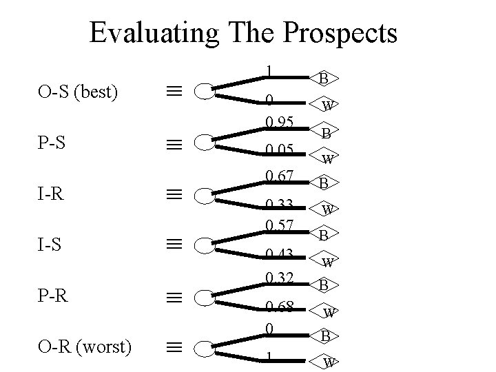
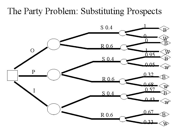
Evaluating The Prospects O-S (best) P-S I-R I-S P-R O-R (worst) 1 0 0. 95 0. 05 0. 67 0. 33 0. 57 0. 43 0. 32 B W B W B 0. 68 0 B 1 W W

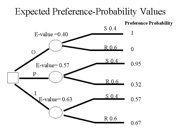
The Party Problem: Adding Probabilities S 0. 4 O R 0. 6 S 0. 4 P R 0. 6 I S 0. 4 R 0. 6

The Party Problem: Substituting Prospects S 0. 4 O R 0. 6 S 0. 4 P R 0. 6 I S 0. 4 R 0. 6 1 0 0 1 0. 95 0. 05 0. 32 0. 68 0. 57 0. 43 B W B W B W 0. 67 B 0. 33 W

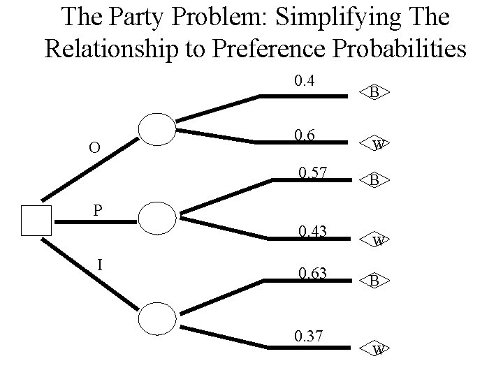
The Party Problem: Simplifying The Relationship to Preference Probabilities 0. 4 O 0. 6 0. 57 B W B P 0. 43 I 0. 63 0. 37 W B W

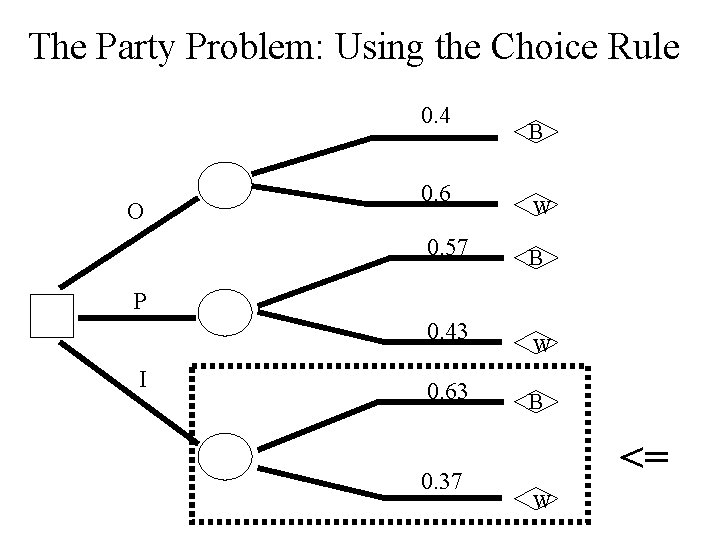
The Party Problem: Using the Choice Rule 0. 4 O 0. 6 0. 57 B W B P 0. 43 I 0. 63 0. 37 W B <= W

Expected Preference-Probability Values E-value =0. 40 O E-value= 0. 57 P I E-value= 0. 63 S 0. 4 Preference Probability 1 R 0. 6 0 S 0. 4 0. 95 R 0. 6 0. 32 S 0. 4 0. 57 R 0. 67

Computation With Decision Trees: Making the Decision • Decision trees are “folded back” to the top most (leftmost, or initial) decision • Computation is performed by averaging expected utility (in this case, preference probability) recursively over tree branches from right to left (bottom up), maximizing utility for every decision made and assuming that this is the expected utility for the subtree that follows the computed decision

(The Value of Information (VI • We often need to decide what would be the next best piece of information to gather (e. g. , within a diagnostic process); that is, what is the best next question to ask (e. g. , what would be the result of a urine culture? ); • Alternatively, we might need to decide how much, if at all, is a paticular additional piece of information worth • The Value of Information (VI) of feature f is the marginal expected utility of an optimal decision made knowing f, compared to making it without knowing f • The net value of information (NVI) of f = VI(f)-cost(f) • NVI is highly useful when deciding what would be the next information item, if any, to investigate

Computing the Value of Information: Requirements • Decision Makers are often faced with the option of getting additional information for a certain cost • To assess the value of additional information to the decision maker, we need a continuous, real valued utility measure, such as money • Thus, we need to map preference probabilities to a monetary scale or an equivalent one (such as time)

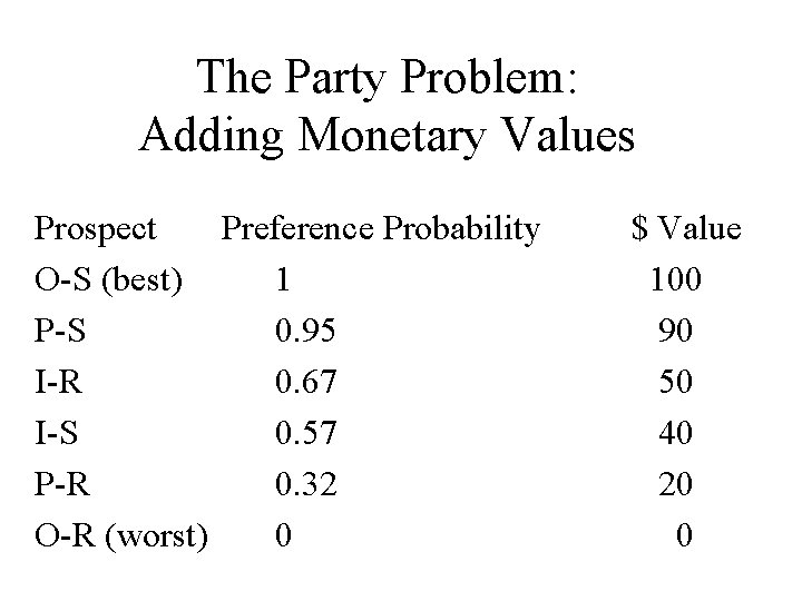
Introducing Monetary Values: Bringing in The Wizard • We ask the decision maker for her willingness to pay for a change from any state to any other state, assuming we have a wizard who can perform the change instantaneously • We can thus create a 1: 1 correspondence between preference probabilities and $ values

The Party Problem: Adding Monetary Values Prospect Preference Probability O-S (best) 1 P-S 0. 95 I-R 0. 67 I-S 0. 57 P-R 0. 32 O-R (worst) 0 $ Value 100 90 50 40 20 0

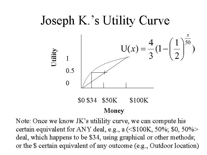
Utility Joseph K. ’s Utility Curve 1 0. 5 + 0 $0 $34 $50 K $100 K Money Note: Once we know JK’s utilility curve, we can compute his certain equivalent for ANY deal, e. g. , a (<$100 K, 50%; $0, 50%> deal, which happens to be $34, using graphical or other methods; or the $ certain equivalent of any outcome (e. g. , Outdoor location)

The Value of Clairvoyance • To compute the value of information, we assume a clairvoyant who knows with certainty all outcomes and always tells the truth • However, clairvoyance has a price! • Thus, the question is, How Much should we pay the clairvoyant for her forecast (e. g. , for telling Joseph K. if it will rain or not)

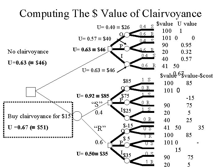
Computing the Value of Clairvoyance • We build a decision tree comparing the optimal decision without clairvoyance to the optimal decision given that the clairvoyant prophesies any of the possible outcomes (in this case, with 100% accuracy) • We need to deduct the cost of clairvoyance from the $ value of all outcomes and role the decision tree back as we did before, to determine the expected value of the decision given clairvoyance (and paying for it!) • We compute e-values using u-values (which represent the decision maker’s utility for each $ value) • At the end (root node) we convert u-values to $ values • We then know whether the clairvoyance is worth its cost

Computing The $ Value of Clairvoyance No clairvoyance U=0. 63 ( $46) U= 0. 40 $26 O U= 0. 57 $40 P U= 0. 63 $46 I “S” Buy clairvoyance for $15 U =0. 67 ( $51) 0. 4 0. 6 U= 0. 63 $46 U= 0. 92 $85 0. 4 0. 6 0. 4 $85 O $75 P I $25 1 S $value U value 100 1 101 0 0 90 0. 95 R 20 0. 32 S 40 0. 57 R 41 50 0. 67$value-$cost $value S R S 0 R 1 S 0 R “R” 0. 6 U= 0. 50 $35 $-15 O $5 P I $35 0 S 1 R 100 85 101 0 -15 90 75 20 5 40 25 41 50 35 100 85 101 0 15 90 75 20 5

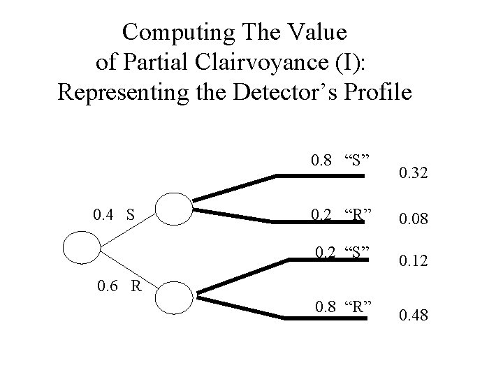
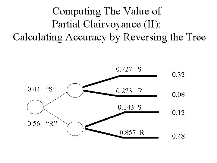
The Value of Partial Clairvoyance • Assume we have a rain detector which, when the weather is going to be sunny or rainy, predicts Rain or Sun 80% of the time, correspondingly; is it worth $10 to use it? • In order to compute the value of an uncertain piece of information, we first need to calculate the probability for rain or sun, given each corresponding prediction of the detector • This involves reversing the tree in which the detector information is usually given, using Bayes theorem

Computing The Value of Partial Clairvoyance (I): Representing the Detector’s Profile 0. 8 “S” 0. 4 S 0. 32 0. 2 “R” 0. 08 0. 2 “S” 0. 12 0. 8 “R” 0. 48 0. 6 R

Computing The Value of Partial Clairvoyance (II): Calculating Accuracy by Reversing the Tree 0. 727 S 0. 44 “S” 0. 273 R 0. 143 S 0. 32 0. 08 0. 12 0. 56 “R” 0. 857 R 0. 48

Computing The Value of Partial Clairvoyance (III): Calculating the Optimal Decision With and Without Clairvoyance • To actually calculate the value of uncertain information, we compare the expected utility of the best decision without the information to the expected utility of the decision with the information, as we did before • We use the distribution of real world states given the semiclairvoyant’s prediction (using our accuracy calculation) • In this particular case (80% accuracy), the value without detector is U = 0. 627, or $45. 83; the value with partial information is U = 0. 615, or $44. 65 • Thus, for Joseph K. , this particular detector is not worth the money

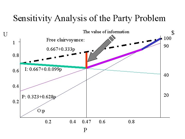
Sensitivity Analysis • The main insights into a decision are often given by an analysis of the influence of the given probabilities and utilities on the final decision and its value • We thus get a sense as to how sensitive the expected utility and optimal decisions are to each parameter, and can focus our attention (and perhaps, further elicitation efforts) on the most important aspects of the problem

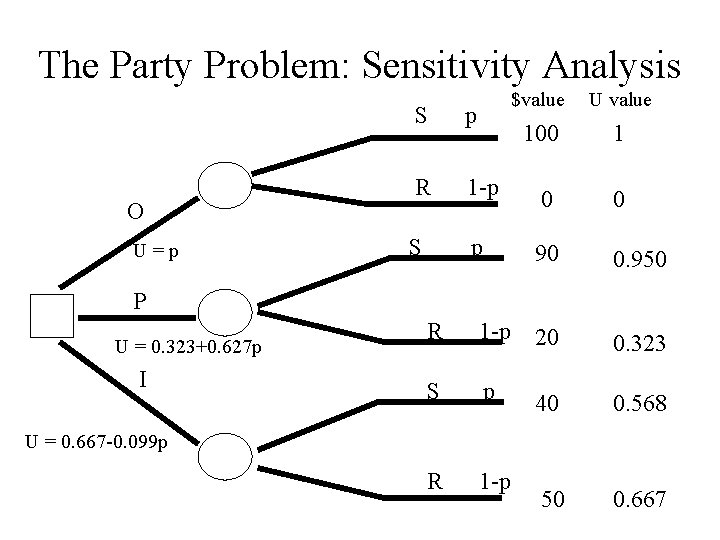
The Party Problem: Sensitivity Analysis O U=p $value U value 100 1 S p R 1 -p 0 0 S p 90 0. 950 P U = 0. 323+0. 627 p I R 1 -p 20 0. 323 S p 40 0. 568 R 1 -p 50 0. 667 U = 0. 667 -0. 099 p

Sensitivity Analysis of the Party Problem The value of information U 100 90 Free clairvoyance: 1 $ 0. 667+0. 333 p 0. 8 0. 6 I: 0. 667+0. 0. 099 p 40 0. 4 0. 2 20 P: 0. 323+0. 628 p O: p 0. 2 0. 47 P 0. 6 0. 8

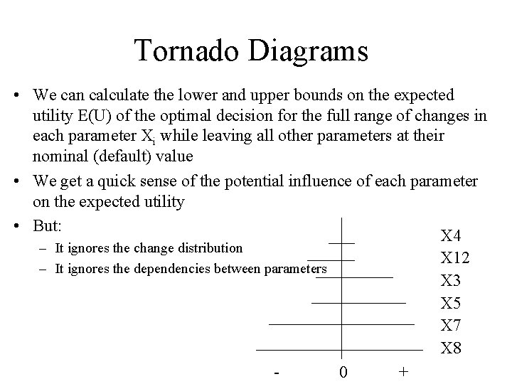
Tornado Diagrams • We can calculate the lower and upper bounds on the expected utility E(U) of the optimal decision for the full range of changes in each parameter Xi while leaving all other parameters at their nominal (default) value • We get a quick sense of the potential influence of each parameter on the expected utility • But: X 4 – It ignores the change distribution X 12 – It ignores the dependencies between parameters X 3 X 5 X 7 X 8 0 +