Judgment and Decision Making in Information Systems Computing

Judgment and Decision Making in Information Systems Computing with Influence Diagrams and the Path. Finder Project Yuval Shahar, M. D. , Ph. D.

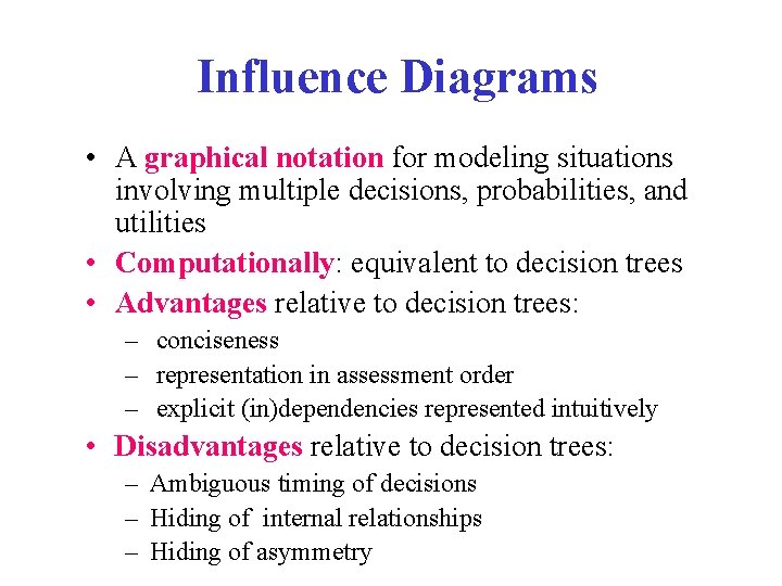
Influence Diagrams • A graphical notation for modeling situations involving multiple decisions, probabilities, and utilities • Computationally: equivalent to decision trees • Advantages relative to decision trees: – conciseness – representation in assessment order – explicit (in)dependencies represented intuitively • Disadvantages relative to decision trees: – Ambiguous timing of decisions – Hiding of internal relationships – Hiding of asymmetry

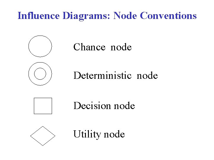
Influence Diagrams: Node Conventions Chance node Deterministic node Decision node Utility node

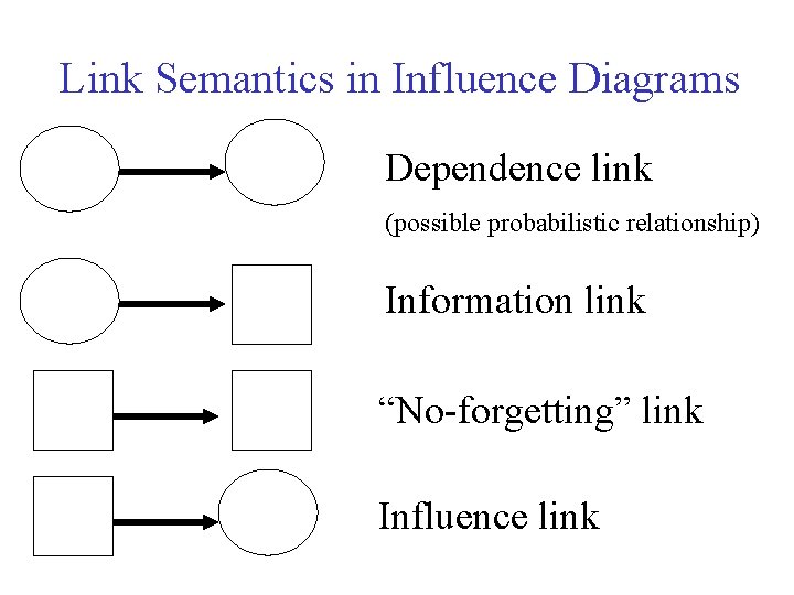
Link Semantics in Influence Diagrams Dependence link (possible probabilistic relationship) Information link “No-forgetting” link Influence link

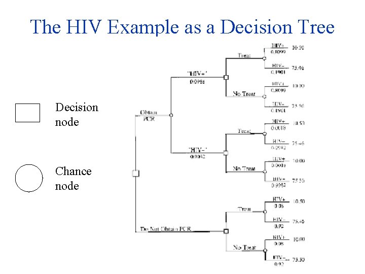
The HIV Example as a Decision Tree Decision node Chance node

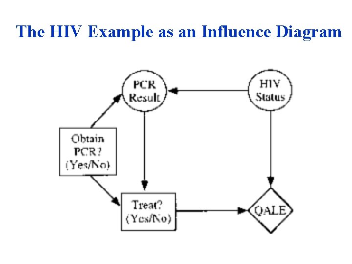
The HIV Example as an Influence Diagram

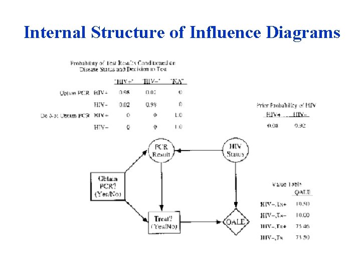
Internal Structure of Influence Diagrams

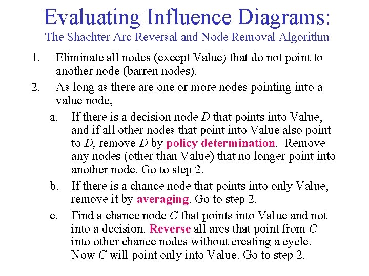
Evaluating Influence Diagrams: The Shachter Arc Reversal and Node Removal Algorithm 1. Eliminate all nodes (except Value) that do not point to another node (barren nodes). 2. As long as there are one or more nodes pointing into a value node, a. If there is a decision node D that points into Value, and if all other nodes that point into Value also point to D, remove D by policy determination. Remove any nodes (other than Value) that no longer point into another node. Go to step 2. b. If there is a chance node that points into only Value, remove it by averaging. Go to step 2. c. Find a chance node C that points into Value and not into a decision. Reverse all arcs that point from C into other chance nodes without creating a cycle. Now C will point only into Value. Go to step 2.

Evaluating Influence Diagrams: Computational Notes • Removal of any type of node involves drawing the arcs from its parent to its child (Value) • In Step 2 a, the decision D pointing into Value has observed all the relevant information (chance outcomes); we can chose the best policy and remove D • In Step 2 b, the outcomes of C are revealed after all decisions were made, so we can average the values (equivalent to folding back a branch of a decision tree) and remove C • In Step 2 b, the outcomes of C are revealed after all decisions were made, but we need to reverse the arcs pointing from it to other chance nodes (by application of Bayes’ theorem) to get an observation order; note that arc reversal might involve adding new arcs, so that the two nodes have the same parents

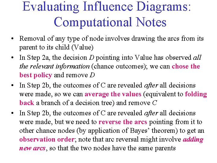
Evaluating the HIV Example (I) Note: We cannot remove any nodes, so we reverse the arc

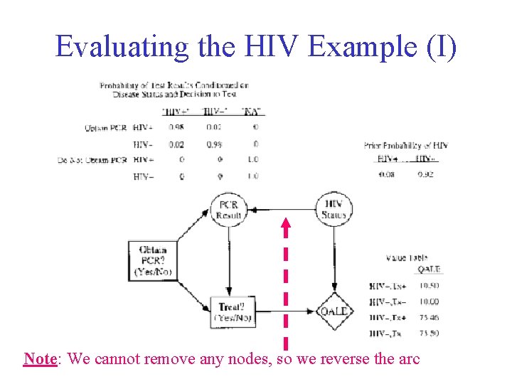
Evaluating the HIV Example (II) Note: “HIV Status” is now conditioned on “Obtain PCR? ” and “PCR Result” by adding an arc from “Obtain PCR? ” and reversing the arcs

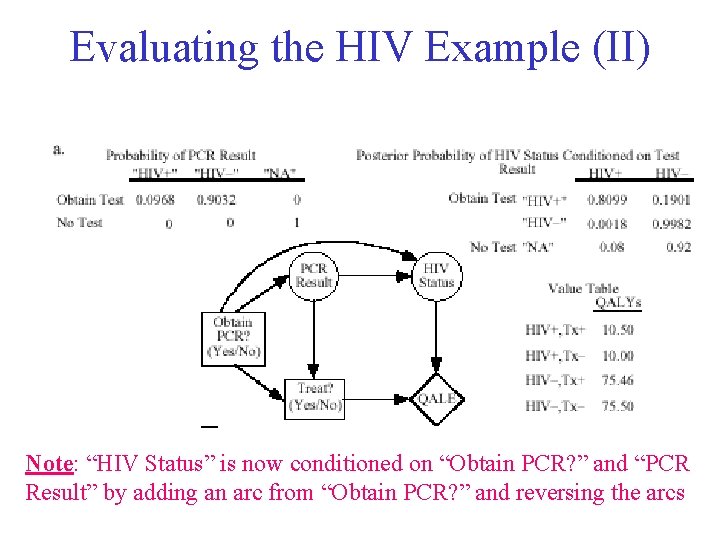
Evaluating the HIV Example (III) Note: “HIV Status” has been removed and Value is conditioned on “Obtain PCR? , ” “PCR Result, ” and “Treat? ” which enables us to remove “? Treat? ” by policy determination for each case

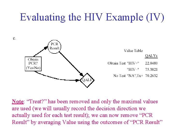
Evaluating the HIV Example (IV) Note: “Treat? ” has been removed and only the maximal values are used (we will usually record the decision direction we actually used for each test result); we can now remove “PCR Result” by averaging Value using the outcomes of “PCR Result”

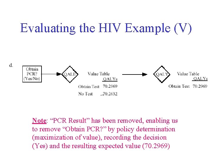
Evaluating the HIV Example (V) Note: “PCR Result” has been removed, enabling us to remove “Obtain PCR? ” by policy determination (maximization of value), recording the decision (Yes) and the resulting expected value (70. 2969)

The Pathfinder Project (Heckerman, Horvitz, Nathwani 1992) • Task and domain: Diagnosis of lymph node biopsy, an important medical problem – Large difference between expert and general pathologist opinions (almost 65%!) • Problems in the domain include – Misrecognition of features (information gathering) – Misintegration of evidence (information processing) • The Pathfinder project focused mainly on assistance in information processing • A Stanford/USC collaboration; eventually commercialized as Intellipath, marketed by the ACP, used as early as 1992 by at least 200 pathology sites

Pathfinder Domain • More than 60 diseases • More than 130 findings, such as: – – – Microscopic immunological molecular biology Laboratory Clinical • Commercial product extended to at least 10 more medical domains

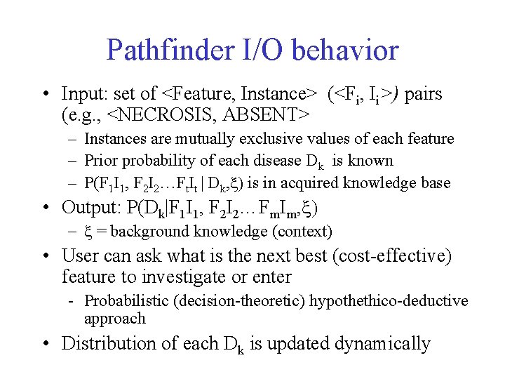
Pathfinder I/O behavior • Input: set of <Feature, Instance> (<Fi, Ii>) pairs (e. g. , <NECROSIS, ABSENT> – Instances are mutually exclusive values of each feature – Prior probability of each disease Dk is known – P(F 1 I 1, F 2 I 2…Ft. It | Dk, x) is in acquired knowledge base • Output: P(Dk|F 1 I 1, F 2 I 2…Fm. Im, x) - x = background knowledge (context) • User can ask what is the next best (cost-effective) feature to investigate or enter - Probabilistic (decision-theoretic) hypothethico-deductive approach • Distribution of each Dk is updated dynamically

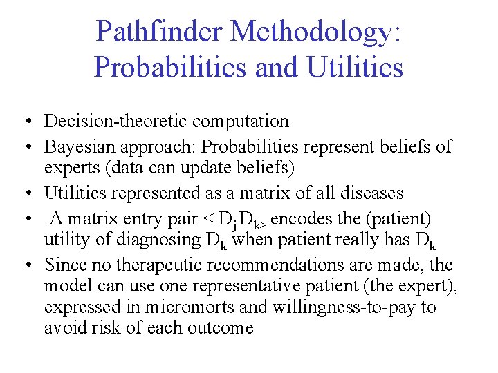
Pathfinder Methodology: Probabilities and Utilities • Decision-theoretic computation • Bayesian approach: Probabilities represent beliefs of experts (data can update beliefs) • Utilities represented as a matrix of all diseases • A matrix entry pair < Dj Dk> encodes the (patient) utility of diagnosing Dk when patient really has Dk • Since no therapeutic recommendations are made, the model can use one representative patient (the expert), expressed in micromorts and willingness-to-pay to avoid risk of each outcome

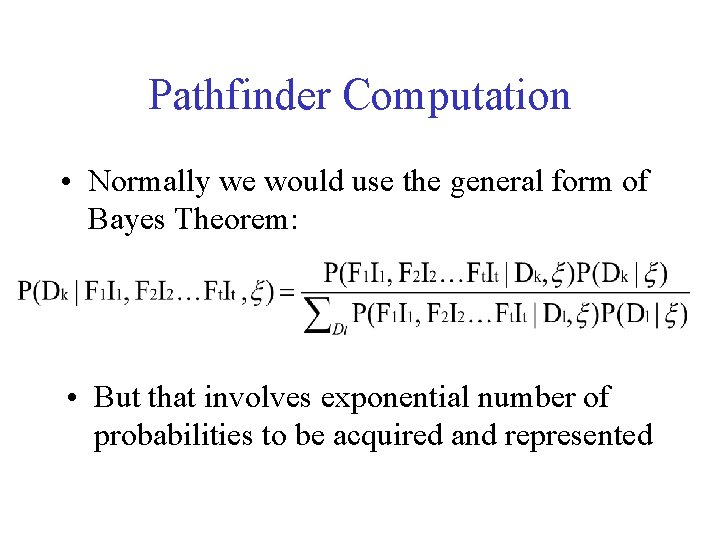
Pathfinder Computation • Normally we would use the general form of Bayes Theorem: • But that involves exponential number of probabilities to be acquired and represented

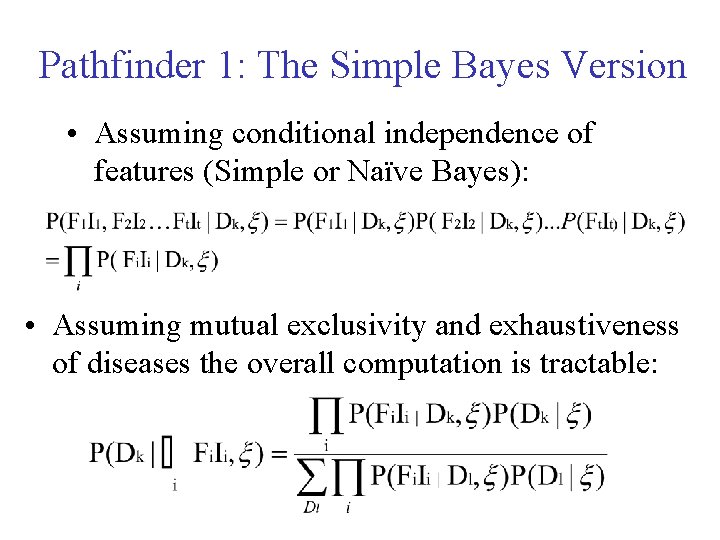
Pathfinder 1: The Simple Bayes Version • Assuming conditional independence of features (Simple or Naïve Bayes): • Assuming mutual exclusivity and exhaustiveness of diseases the overall computation is tractable:

Pathfinder 2: The Belief Network Version • Mutual exclusivity and exhaustiveness of diseases is reasonable in lymphnode pathology – Single disease per examined lymph node – Large, exhaustive knowledge base • Conditional independence is less reasonable and can lead to erroneous conclusions • The simple Bayes representation of Pathfinder 1 was therefore enhanced to a belief network in Pathfinder 2 which included explicit dependencies between different features, still taking advantage of any explicit global and conditional independencies

Decision-Theoretic Diagnosis • Using the utility matrix and given observations f, the expected diagnostic utility using f is averaged over all diagnoses: – EU(Dk(f)) = Sj. P(Dj| f)U(Dj, Dk) • Thus, Dx(f) = ARGMAXk [EU(Dk (f)) • However, since the diagnosis is sensitive to the utility model, Pathfinder does not recommend it, only the probabilities P(Dk |f)

Value of Information (VI) • We often need to decide what would be the next best diagnostic test to perform—for example, the next best blood test or even the best next question to ask • Recall: The Value of Information (VI) of feature f is the marginal expected utility of an optimal decision made knowing f, compared to making it without knowing f • The net value of information (NVI) of f = VI(f)-cost(f) • NVI is highly useful for deciding what would be the next test, if any, to perform, in a diagnostic setting

Pathfinder: Gathering Information • Next best feature to observe is recommended using a myopic approximation, which considers only up to one single feature to be observed • The feature chosen maximizes EU given that a diagnosis would be made after observing it • Feature f is chosen that maximizes NVI(f) • Although myopic approximation could backfire, in practice it works well – especially when U(Dj, Dk) =is set to 0 if one of the diseases is malignant and the other benign, and set to 1 if they are both malignant or both benign

Pathfinder 2: Knowledge Acquisition • To facilitate acquisition of multiple probabilities, a Similarity Network model was developed • Using similarity networks, an expert creates multiple small belief networks, representing 2 or more diseases that are difficult to distinguish • The local belief networks are then unified into a global belief network, preserving soundness • The graphical interface also allows partitioning of diseases into sets, relative to each set some feature is independent, thus further assisting in the construction

Pathfinder 1 and 2: Evaluation • Pathfinder 1 was compared to Pathfinder 2 using 53 cases, a new user, and a thorough analysis of each case – Diagnostic accuracy of PF 2 is greater than that of PF 1 (gold standard: the main domain expert’s distribution and his assessment on a scale of 1 to 10) – Difference is due to better probabilistic representation (better acquisition and inference) – Cost of constructing PF 2 rather than PF 1 is justified by the improvements, (measure: the utility of the diagnosis) – PF 2 is at least as good as the main domain expert, with respect to diagnostic accuracy