Judgment and Decision Making in Information Systems Utility

Judgment and Decision Making in Information Systems Utility Functions, Utility Elicitation, and Risk Attitudes. Yuval Shahar, M. D. , Ph. D

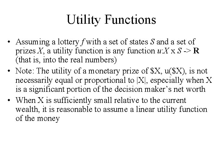
Utility Functions • Assuming a lottery f with a set of states S and a set of prizes X, a utility function is any function u: X x S -> R (that is, into the real numbers) • Note: The utility of a monetary prize of $X, u($X), is not necessarily equal or proportional to |X|, especially when X is a significant portion of the decision maker’s net worth • When X is sufficiently small relative to the current wealth, it is reasonable to assume a linear utility function of the money

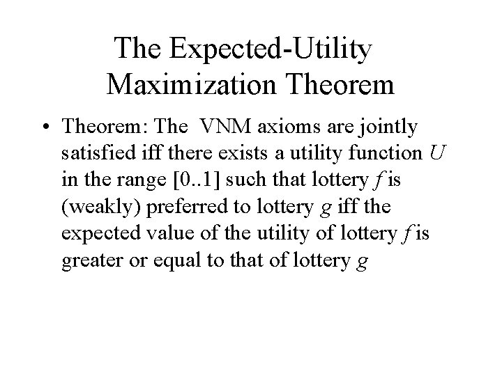
The Expected-Utility Maximization Theorem • Theorem: The VNM axioms are jointly satisfied iff there exists a utility function U in the range [0. . 1] such that lottery f is (weakly) preferred to lottery g iff the expected value of the utility of lottery f is greater or equal to that of lottery g

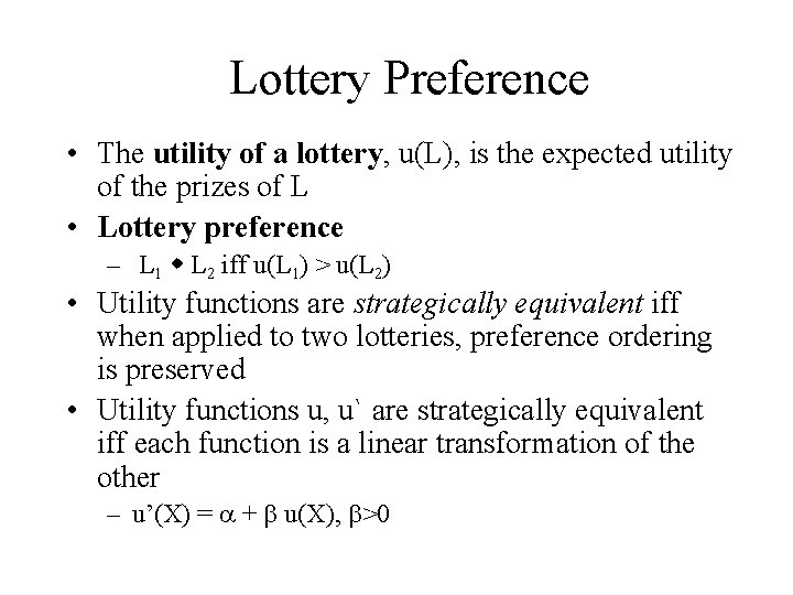
Lottery Preference • The utility of a lottery, u(L), is the expected utility of the prizes of L • Lottery preference – L 1 L 2 iff u(L 1) > u(L 2) • Utility functions are strategically equivalent iff when applied to two lotteries, preference ordering is preserved • Utility functions u, u` are strategically equivalent iff each function is a linear transformation of the other – u’(X) = + u(X), >0

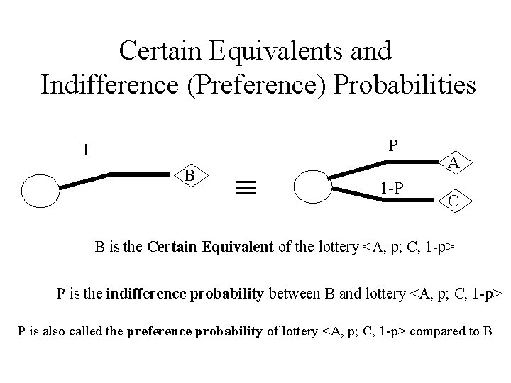
Certain Equivalents and Indifference (Preference) Probabilities P 1 B 1 -P A C B is the Certain Equivalent of the lottery <A, p; C, 1 -p> P is the indifference probability between B and lottery <A, p; C, 1 -p> P is also called the preference probability of lottery <A, p; C, 1 -p> compared to B

The Civil Lawsuit Case • Consider the option of either – A: paying $50, 000 and gambling • (A 1) That the jury will decide in your favor and give you $1 M (net gain: $950 K), or • (A 2) That you lose the case (and the $50 K) – B: settling out of court for $650, 000 for sure • => Utility functions are not likely to be linear for significant losses or wins!

Elicitation of Utility Functions • Utilities are individual and subjective • Utilities need to be elicited from the decision maker to support their decision • There are two basic approaches: – Determining the indifference probabilities, given a certain equivalent – Determining a certain equivalent, given an indifference probability

Utility Elicitation (I): Determining the Indifference Probability • Ask the decision maker: – Given outcomes R 1 (best), R 1 (worst), and potential certain equivalent Req, what is the indifference probability p of the deal < R 1, p; R 0, 1 -p> relative to Req. That is, U (Req) = p • Search for p iteratively by limiting the interval containing it from both ends in “ping pong” fashion (e. g. 99%, 1%, 90%, 10%…) until the indifference probability is found • Note: For non-continuous outcomes such as {Win, Draw, Lose}, using linear (convex) combinations of the value of the outcome to express the value of the certain equivalent would be meaningless

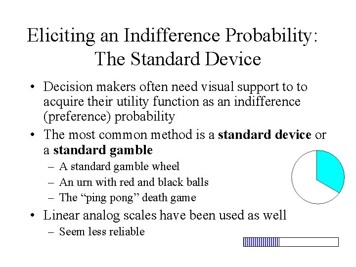
Eliciting an Indifference Probability: The Standard Device • Decision makers often need visual support to to acquire their utility function as an indifference (preference) probability • The most common method is a standard device or a standard gamble – A standard gamble wheel – An urn with red and black balls – The “ping pong” death game • Linear analog scales have been used as well – Seem less reliable

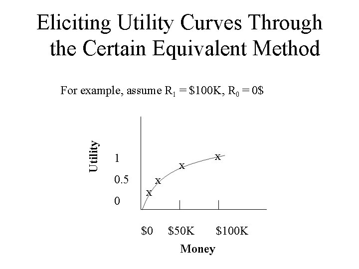
Utility Elicitation (II): Determining the Certain Equivalent • Assume u(R 0) = 0, u(R 1) = 1 • Ask the decision maker: – What would be your certain equivalent for a deal of < R 1, 50%; R 0, 50%> ? Assume it is Req, u(Req) = 0. 5 • Ask iteratively for the certain equivalent of the deal < R 1, 50%; Req, 50%>, the deal < Req, 50%; R 0, 50%> , etc. The utility of these intermediate certain equivalents must be 0. 75, 0. 25, etc. • Continue until utility curve is sufficiently clear • Note: Useful (only) for continuous outcomes that can be meaningfully combined in linear fashion

Eliciting Utility Curves Through the Certain Equivalent Method Utility For example, assume R 1 = $100 K, R 0 = 0$ 1 0. 5 0 x x $50 K $100 K Money

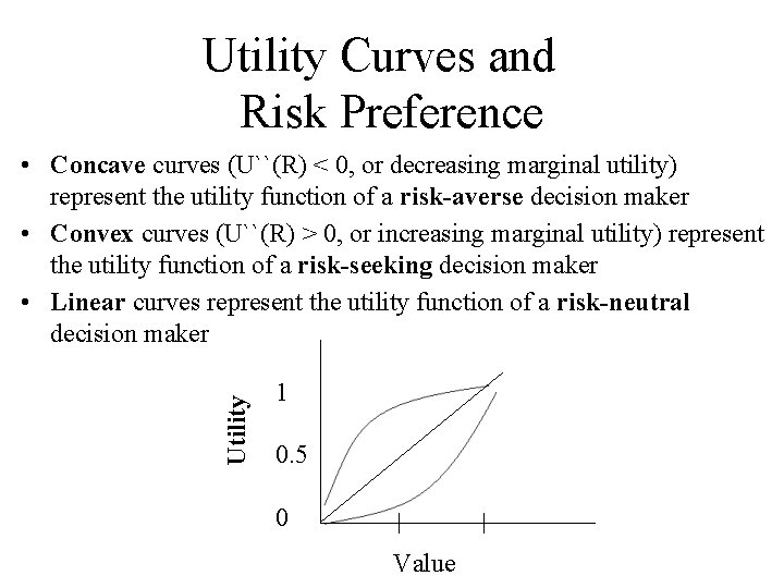
Utility Curves and Risk Preference Utility • Concave curves (U``(R) < 0, or decreasing marginal utility) represent the utility function of a risk-averse decision maker • Convex curves (U``(R) > 0, or increasing marginal utility) represent the utility function of a risk-seeking decision maker • Linear curves represent the utility function of a risk-neutral decision maker 1 0. 5 0 Value

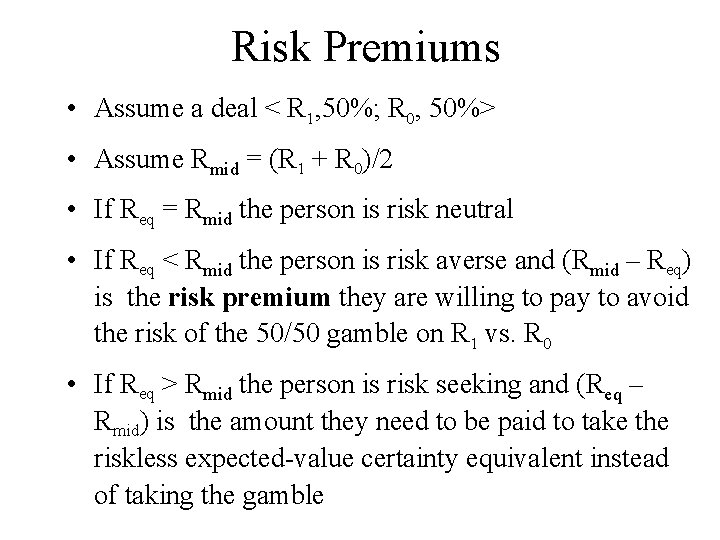
Risk Premiums • Assume a deal < R 1, 50%; R 0, 50%> • Assume Rmid = (R 1 + R 0)/2 • If Req = Rmid the person is risk neutral • If Req < Rmid the person is risk averse and (Rmid – Req) is the risk premium they are willing to pay to avoid the risk of the 50/50 gamble on R 1 vs. R 0 • If Req > Rmid the person is risk seeking and (Req – Rmid) is the amount they need to be paid to take the riskless expected-value certainty equivalent instead of taking the gamble

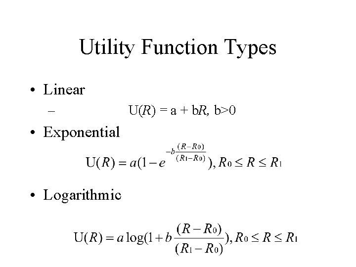
Utility Function Types • Linear – • Exponential • Logarithmic U(R) = a + b. R, b>0

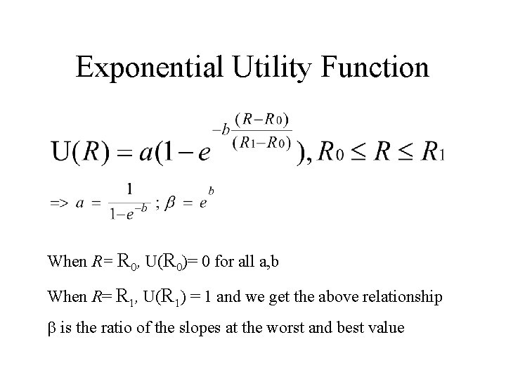
Exponential Utility Function When R= R 0, U(R 0)= 0 for all a, b When R= R 1, U(R 1) = 1 and we get the above relationship is the ratio of the slopes at the worst and best value

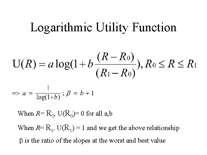
Logarithmic Utility Function When R= R 0, U(R 0)= 0 for all a, b When R= R 1, U(R 1) = 1 and we get the above relationship is the ratio of the slopes at the worst and best value

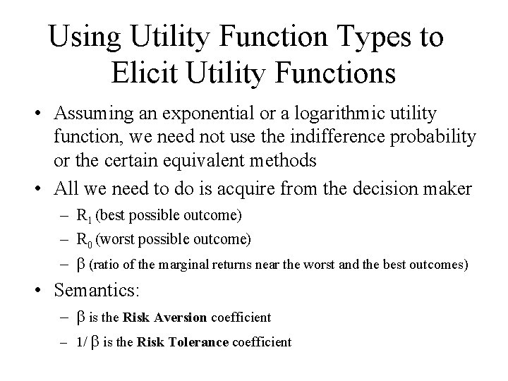
Using Utility Function Types to Elicit Utility Functions • Assuming an exponential or a logarithmic utility function, we need not use the indifference probability or the certain equivalent methods • All we need to do is acquire from the decision maker – R 1 (best possible outcome) – R 0 (worst possible outcome) – (ratio of the marginal returns near the worst and the best outcomes) • Semantics: – is the Risk Aversion coefficient – 1/ is the Risk Tolerance coefficient

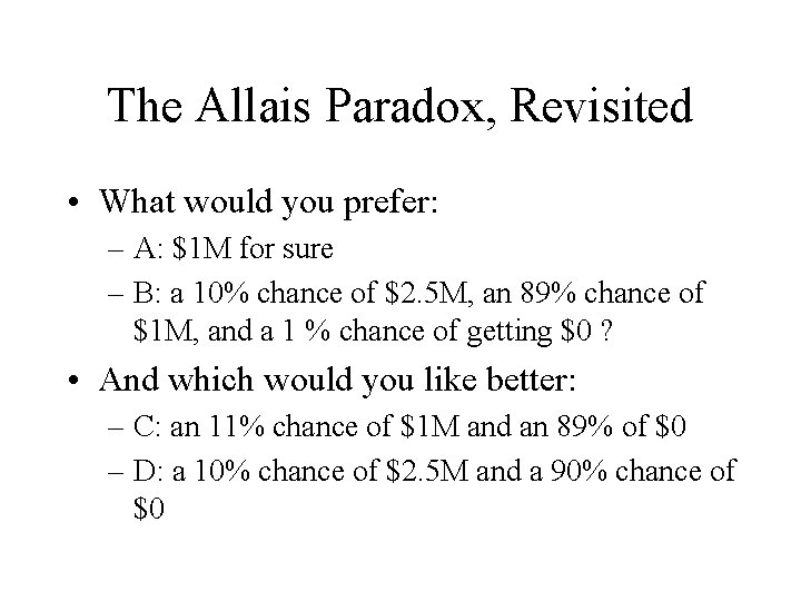
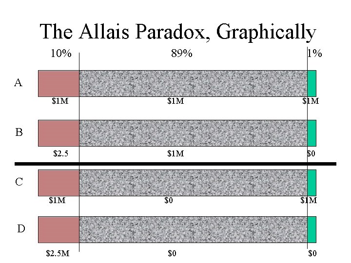
The Allais Paradox, Revisited • What would you prefer: – A: $1 M for sure – B: a 10% chance of $2. 5 M, an 89% chance of $1 M, and a 1 % chance of getting $0 ? • And which would you like better: – C: an 11% chance of $1 M and an 89% of $0 – D: a 10% chance of $2. 5 M and a 90% chance of $0

The Allais Paradox, Graphically 10% 89% 1% A $1 M $1 M $2. 5 $1 M $0 B C $1 M $0 $1 M D $2. 5 M $0 $0