INTRODUCTION TO CLINICAL RESEARCH Survival Analysis Getting Started

INTRODUCTION TO CLINICAL RESEARCH Survival Analysis – Getting Started Karen Bandeen-Roche, Ph. D. July 20, 2010

Acknowledgements • Scott Zeger • Marie Diener-West • ICTR Leadership / Team July 2010 JHU Intro to Clinical Research 2

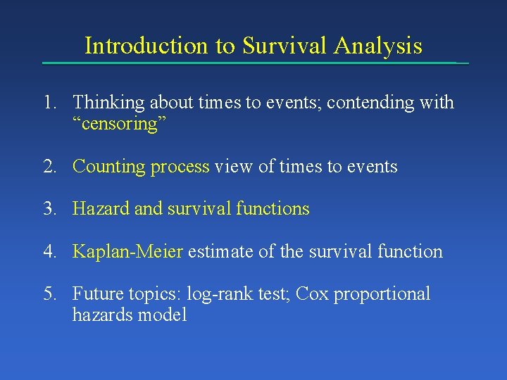
Introduction to Survival Analysis 1. Thinking about times to events; contending with “censoring” 2. Counting process view of times to events 3. Hazard and survival functions 4. Kaplan-Meier estimate of the survival function 5. Future topics: log-rank test; Cox proportional hazards model

“Survival Analysis” • Approach and methods for analyzing times to events • Events not necessarily deaths (“survival” is historical term) • Need special methods to deal with “censoring”

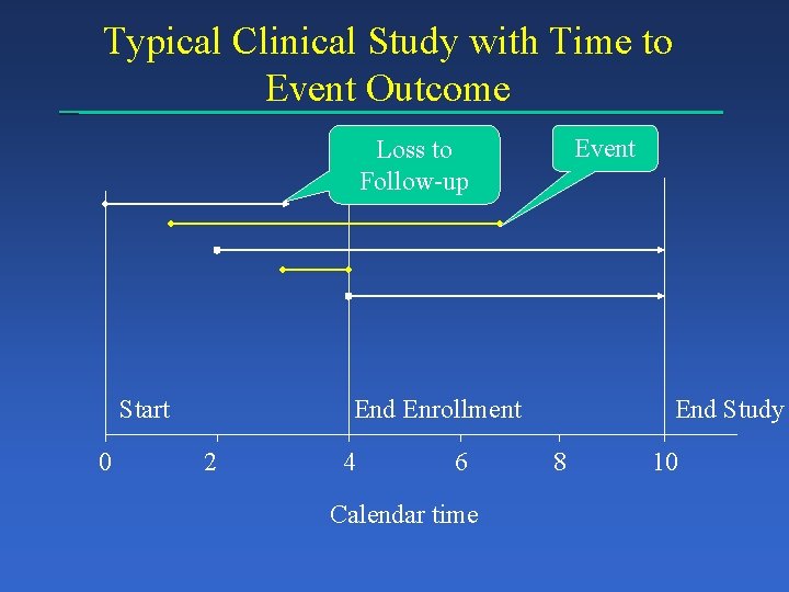
Typical Clinical Study with Time to Event Outcome Event Loss to Follow-up Start 0 End Enrollment 2 4 6 Calendar time End Study 8 10

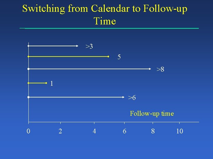
Switching from Calendar to Follow-up Time >3 5 >8 1 >6 Follow-up time 0 2 4 6 8 10

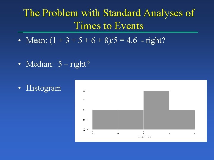
The Problem with Standard Analyses of Times to Events • Mean: (1 + 3 + 5 + 6 + 8)/5 = 4. 6 - right? • Median: 5 – right? • Histogram

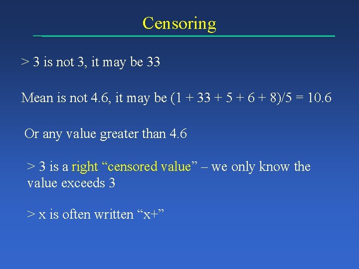
Censoring > 3 is not 3, it may be 33 Mean is not 4. 6, it may be (1 + 33 + 5 + 6 + 8)/5 = 10. 6 Or any value greater than 4. 6 > 3 is a right “censored value” – we only know the value exceeds 3 > x is often written “x+”

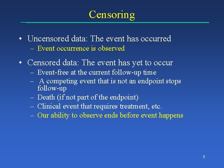
Censoring • Uncensored data: The event has occurred – Event occurrence is observed • Censored data: The event has yet to occur – Event-free at the current follow-up time – A competing event that is not an endpoint stops follow-up – Death (if not part of the endpoint) – Clinical event that requires treatment, etc. – Our ability to observe ends before event happens 9

Contending with Censored Data Standard statistical methods do not work for censored data We need to think of times to events as a natural history in time, not just a single number Issue: If no events are reported in the interval from last follow-up to “now”, need to choose between: No news is good news? No news is no news?

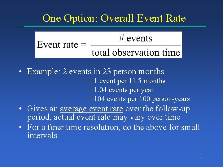
One Option: Overall Event Rate • Example: 2 events in 23 person months = 1 event per 11. 5 months = 1. 04 events per year = 104 events per 100 person-years • Gives an average event rate over the follow-up period; actual event rate may vary over time • For a finer time resolution, do the above for small intervals 11

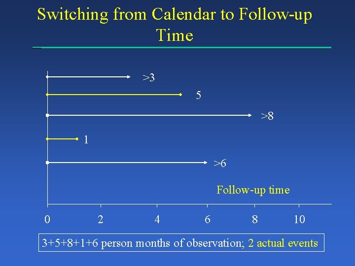
Switching from Calendar to Follow-up Time >3 5 >8 1 >6 Follow-up time 0 2 4 6 8 10 3+5+8+1+6 person months of observation; 2 actual events

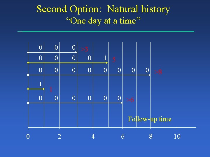
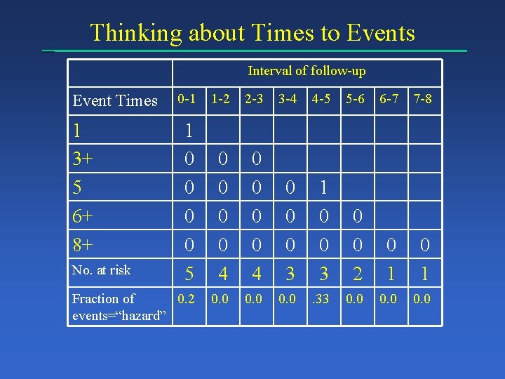
Second Option: Natural history “One day at a time” 0 0 0 >3 0 0 0 1 5 0 0 0 1 0 0 0 >8 1 0 >6 Follow-up time 0 2 4 6 8 10

Thinking about Times to Events Interval of follow-up Event Times 1 3+ 5 6+ 8+ No. at risk 0 -1 1 -2 2 -3 3 -4 4 -5 5 -6 6 -7 7 -8 1 0 0 5 0 0 0 0 4 0 0 0 3 1 0 0 3 0 0 2 0 1 0. 0 . 33 0. 0 Fraction of 0. 2 events=“hazard”

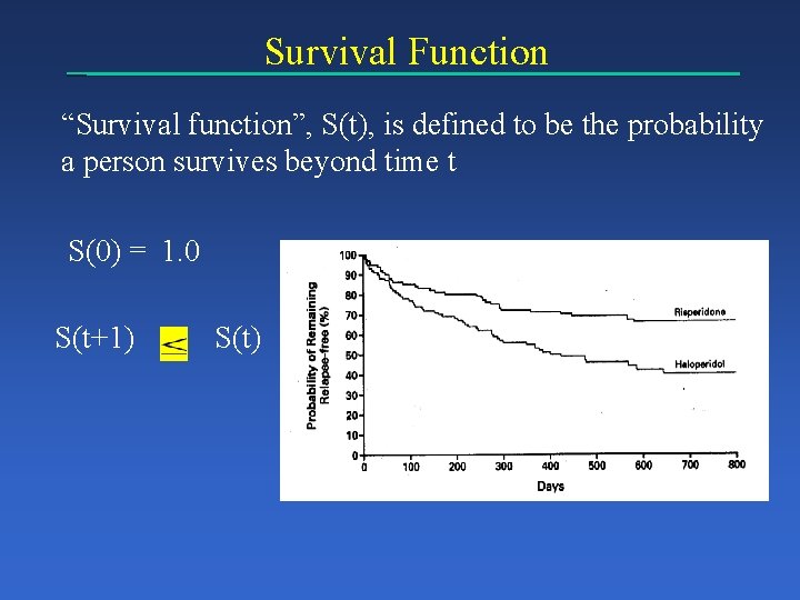
Survival Function “Survival function”, S(t), is defined to be the probability a person survives beyond time t S(0) = 1. 0 S(t+1) S(t)

Hazard Function • Hazard at time t, h(t), is the probability per unit time of having the event in a small interval around time t • Force of mortality • ~ Pr{event in (t, t+dt)}/dt • Need not be between 0 and 1 because it is per unit time • h(t) ~ {S(t)-S(t+dt)}/{S(t) dt}

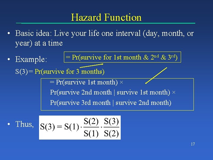
Hazard Function • Basic idea: Live your life one interval (day, month, or year) at a time • Example: = Pr(survive for 1 st month & 2 nd & 3 rd) S(3) = Pr(survive for 3 months) = Pr(survive 1 st month) × Pr(survive 2 nd month | survive 1 st month) × Pr(survive 3 rd month | survive 2 nd month) • Thus, 17

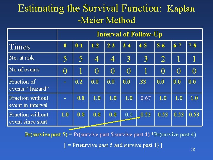
Estimating the Survival Function: Kaplan -Meier Method Interval of Follow-Up Times 0 0 -1 1 -2 2 -3 3 -4 4 -5 5 -6 6 -7 7 -8 No. at risk 5 0 5 1 4 0 3 0 3 1 2 0 1 0 Fraction of events=“hazard” - 0. 2 0. 0 . 33 0. 0 Fraction without event in interval - 0. 8 1. 0 0. 67 1. 0 Fraction without event since start 1. 0 0. 8 0. 53 No of events 1. 0 Pr(survive past 5) = Pr(survive past 5|survive past 4) *Pr(survive past 4) [ = Pr(survive past 5 and survive past 4) ] 18

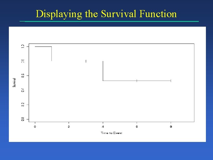
Displaying the Survival Function

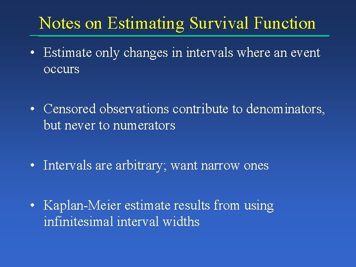
Notes on Estimating Survival Function • Estimate only changes in intervals where an event occurs • Censored observations contribute to denominators, but never to numerators • Intervals are arbitrary; want narrow ones • Kaplan-Meier estimate results from using infinitesimal interval widths

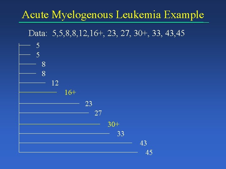
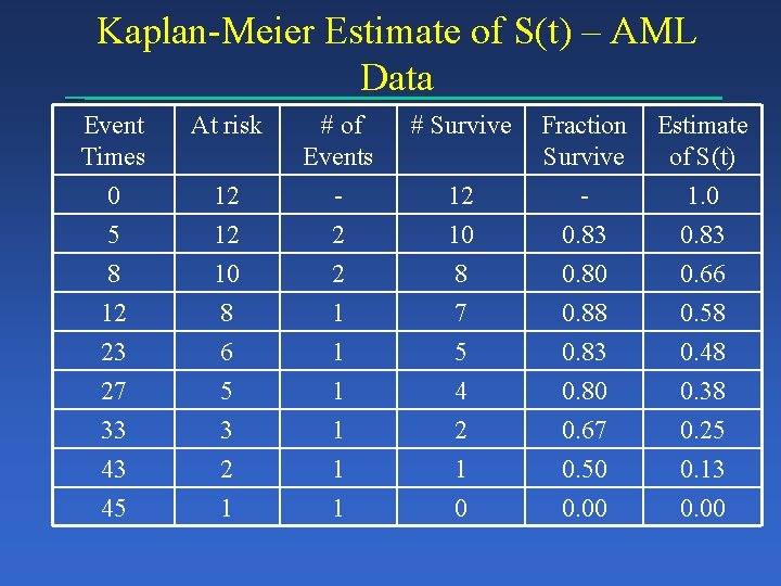
Acute Myelogenous Leukemia Example Data: 5, 5, 8, 8, 12, 16+, 23, 27, 30+, 33, 45 5 5 8 8 12 16+ 23 27 30+ 33 43 45

Kaplan-Meier Estimate of S(t) – AML Data Event Times 0 5 At risk # Survive 12 12 # of Events 2 8 12 23 27 33 43 45 12 10 Fraction Survive 0. 83 Estimate of S(t) 1. 0 0. 83 10 8 6 5 3 2 1 1 1 1 8 7 5 4 2 1 0 0. 88 0. 83 0. 80 0. 67 0. 50 0. 00 0. 66 0. 58 0. 48 0. 38 0. 25 0. 13 0. 00

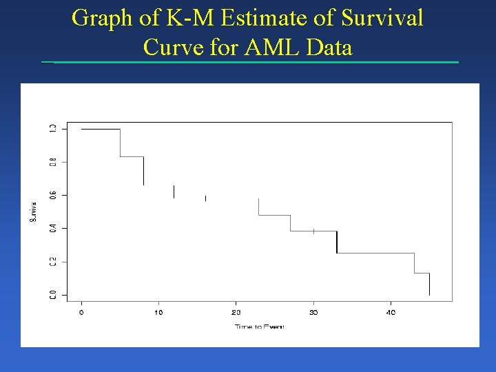
Graph of K-M Estimate of Survival Curve for AML Data

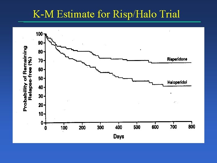
K-M Estimate for Risp/Halo Trial

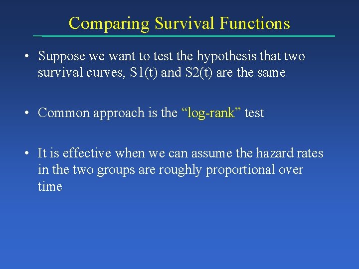
Comparing Survival Functions • Suppose we want to test the hypothesis that two survival curves, S 1(t) and S 2(t) are the same • Common approach is the “log-rank” test • It is effective when we can assume the hazard rates in the two groups are roughly proportional over time

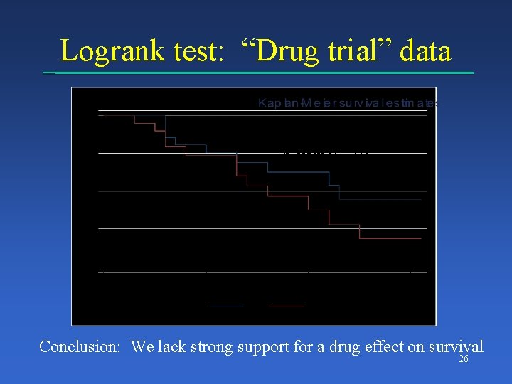
Logrank test: “Drug trial” data Logrank: 1. 72 p-value: . 19 Conclusion: We lack strong support for a drug effect on survival 26

Comparing Survival Functions • Suppose we want to test the hypothesis that two survival curves, S 1(t) and S 2(t) are the same • Common approach is the “log-rank” test • It is effective when we can assume the hazard rates in the two groups are roughly proportional over time • Regression analysis—“Cox” model: more to come

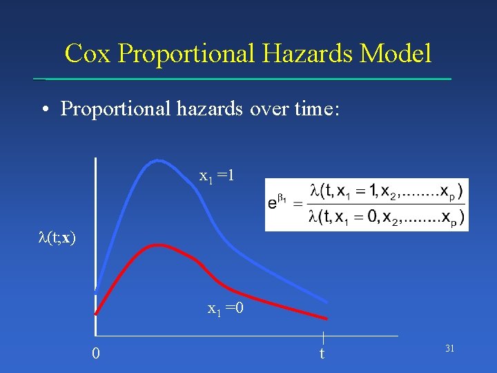
Regression Analysis for Times to Events • Cox proportional hazards model • Hazard of an event is the product of two terms – Baseline hazard, h(t), that depends on time, t – Relative risk, rr(x) that depends on predictor variables, x, but not time • Each person’s hazard varies over time in the same way, but can be higher or lower depending on their predictor variables x 28

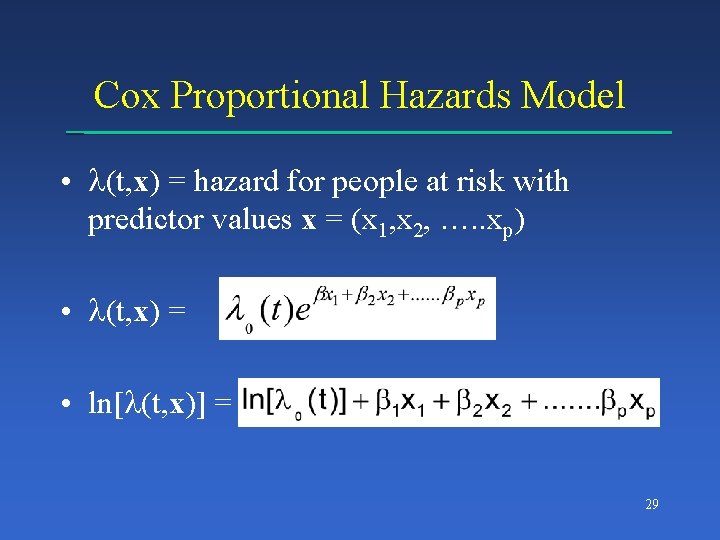
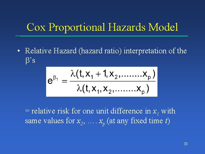
Cox Proportional Hazards Model • (t, x) = hazard for people at risk with predictor values x = (x 1, x 2, …. . xp) • (t, x) = • ln[ (t, x)] = 29

Cox Proportional Hazards Model • Relative Hazard (hazard ratio) interpretation of the ’s = relative risk for one unit difference in x 1 with same values for x 2, …. xp (at any fixed time t) 30

Cox Proportional Hazards Model • Proportional hazards over time: x 1 =1 (t; x) x 1 =0 0 t 31

Main Points Once Again • Time to event data can be censored because every person does not necessarily have the event during the study • Think of time to event as a natural history, that is 0 before the event and then switches to 1 when the event occurs; analysis counts the events • Survival function, S(t), is the probability a person’s event occurs after each time t

Main Points Once Again • Kaplan-Meier estimator of the survival function is a product of interval-specific survival probabilities • Hazard function, h(t), is the risk per unit time of having the event for a person who is at risk (not previously had event) • Logrank tests evaluate differences among survival in population subgroups • Cox model used for regression for survival data