Intelligent Systems AI2 Computer Science cpsc 422 Lecture

Intelligent Systems (AI-2) Computer Science cpsc 422, Lecture 16 Oct, 16, 2015 CPSC 422, Lecture 16 Slide 1

Lecture Overview Probabilistic temporal Inferences • Filtering • Prediction • Smoothing (forward-backward) • Most Likely Sequence of States (Viterbi) • Approx. Inference In Temporal Models (Particle Filtering) CPSC 422, Lecture 16 2

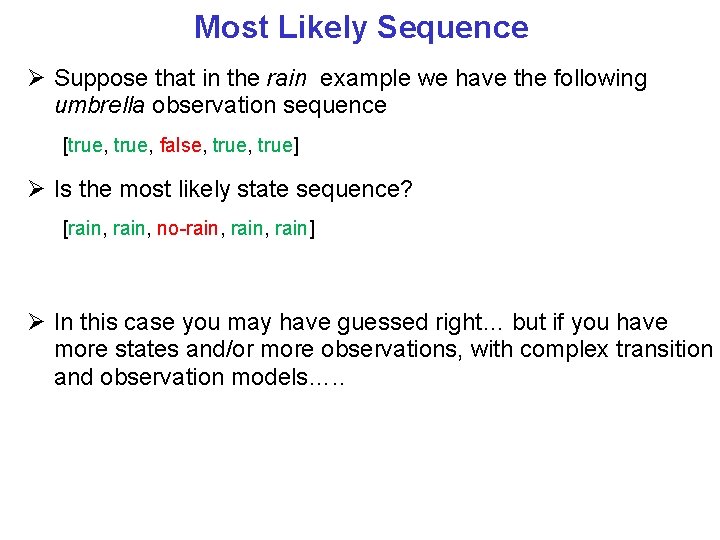
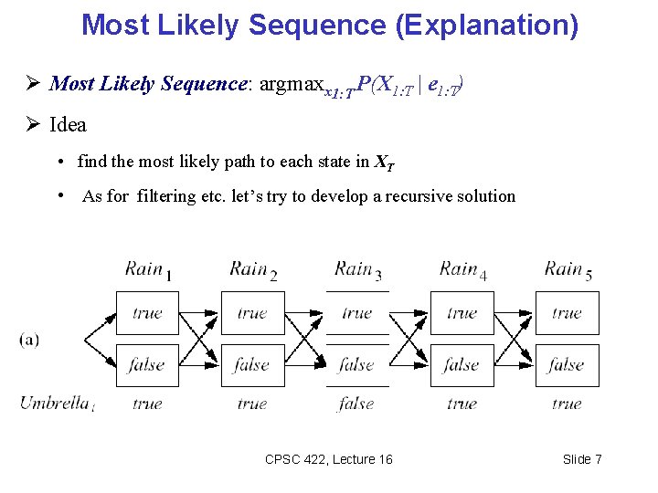
Most Likely Sequence Suppose that in the rain example we have the following umbrella observation sequence [true, false, true] Is the most likely state sequence? [rain, no-rain, rain] In this case you may have guessed right… but if you have more states and/or more observations, with complex transition and observation models…. .

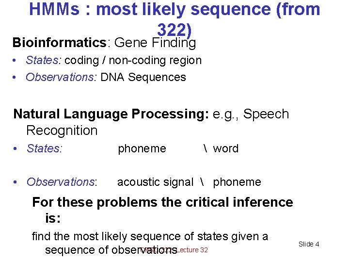
HMMs : most likely sequence (from 322) Bioinformatics: Gene Finding • States: coding / non-coding region • Observations: DNA Sequences Natural Language Processing: e. g. , Speech Recognition • States: phoneme • Observations: acoustic signal phoneme word For these problems the critical inference is: find the most likely sequence of states given a CPSC 322, Lecture 32 sequence of observations Slide 4

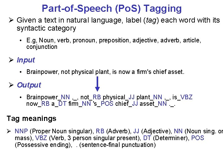
Part-of-Speech (Po. S) Tagging Given a text in natural language, label (tag) each word with its syntactic category • E. g, Noun, verb, pronoun, preposition, adjective, adverb, article, conjunction Input • Brainpower, not physical plant, is now a firm's chief asset. Output • Brainpower_NN , _, not_RB physical_JJ plant_NN , _, is_VBZ now_RB a_DT firm_NN 's_POS chief_JJ asset_NN. _. Tag meanings NNP (Proper Noun singular), RB (Adverb), JJ (Adjective), NN (Noun sing. or mass), VBZ (Verb, 3 person singular present), DT (Determiner), POS (Possessive ending), . (sentence-final punctuation)

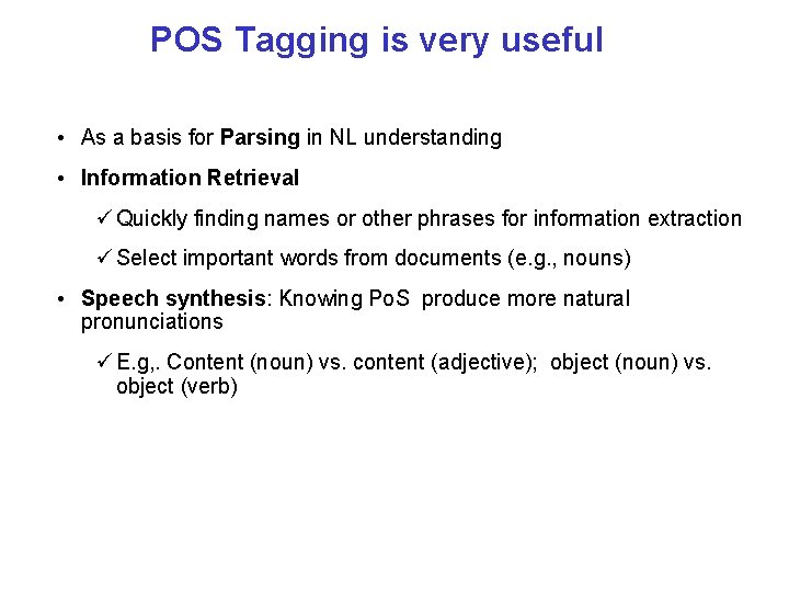
POS Tagging is very useful • As a basis for Parsing in NL understanding • Information Retrieval Quickly finding names or other phrases for information extraction Select important words from documents (e. g. , nouns) • Speech synthesis: Knowing Po. S produce more natural pronunciations E. g, . Content (noun) vs. content (adjective); object (noun) vs. object (verb)

Most Likely Sequence (Explanation) Most Likely Sequence: argmaxx 1: T P(X 1: T | e 1: T) Idea • find the most likely path to each state in XT • As for filtering etc. let’s try to develop a recursive solution CPSC 422, Lecture 16 Slide 7

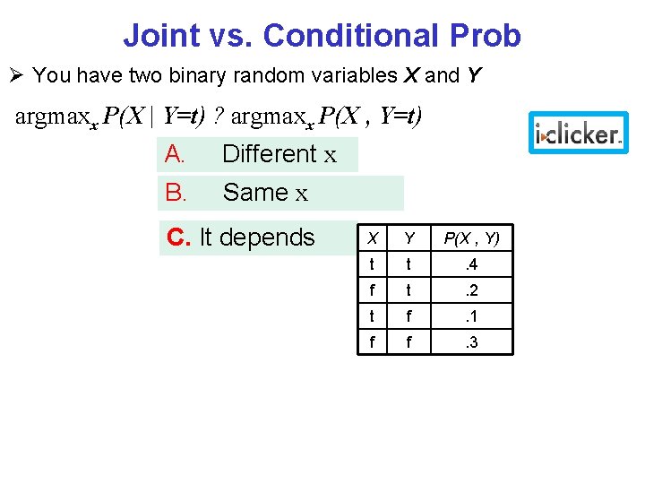
Joint vs. Conditional Prob You have two binary random variables X and Y argmaxx P(X | Y=t) ? argmaxx P(X , Y=t) A. Different x B. Same x C. It depends X Y P(X , Y) t t . 4 f t . 2 t f . 1 f f . 3

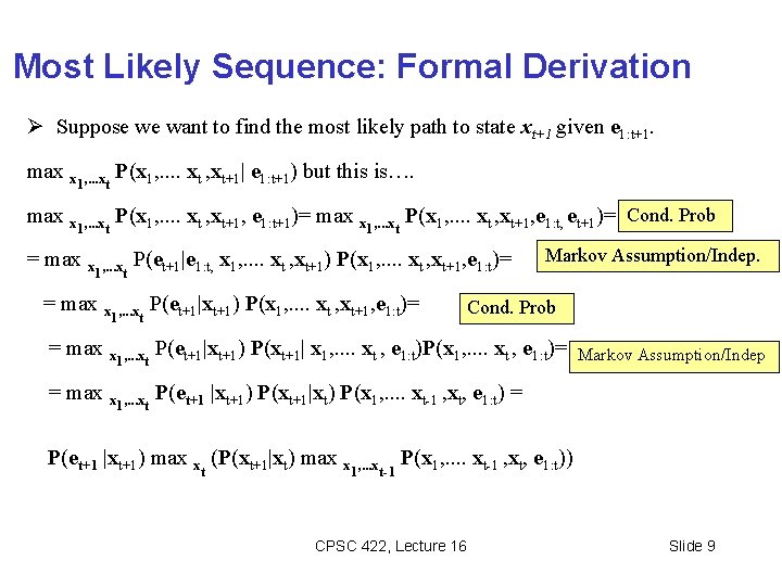
Most Likely Sequence: Formal Derivation Suppose we want to find the most likely path to state xt+1 given e 1: t+1. max x 1, . . . xt P(x 1, . . xt , xt+1| e 1: t+1) but this is…. max x 1, . . . xt P(x 1, . . xt , xt+1, e 1: t+1)= max x 1, . . . xt P(x 1, . . xt , xt+1, e 1: t, et+1)= Cond. Prob P(et+1|e 1: t, x 1, . . xt , xt+1) P(x 1, . . xt , xt+1, e 1: t)= 1, . . . xt P(et+1|xt+1) P(x 1, . . xt , xt+1, e 1: t)= Markov Assumption/Indep. Cond. Prob = max x 1, . . . xt P(et+1|xt+1) P(xt+1| x 1, . . xt , e 1: t)P(x 1, . . xt , e 1: t)= = max x 1, . . . xt P(et+1 |xt+1) P(xt+1|xt) P(x 1, . . xt-1 , xt, e 1: t) = P(et+1 |xt+1) max x (P(xt+1|xt) max x t 1, . . . xt-1 Markov Assumption/Indep P(x 1, . . xt-1 , xt, e 1: t)) CPSC 422, Lecture 16 Slide 9

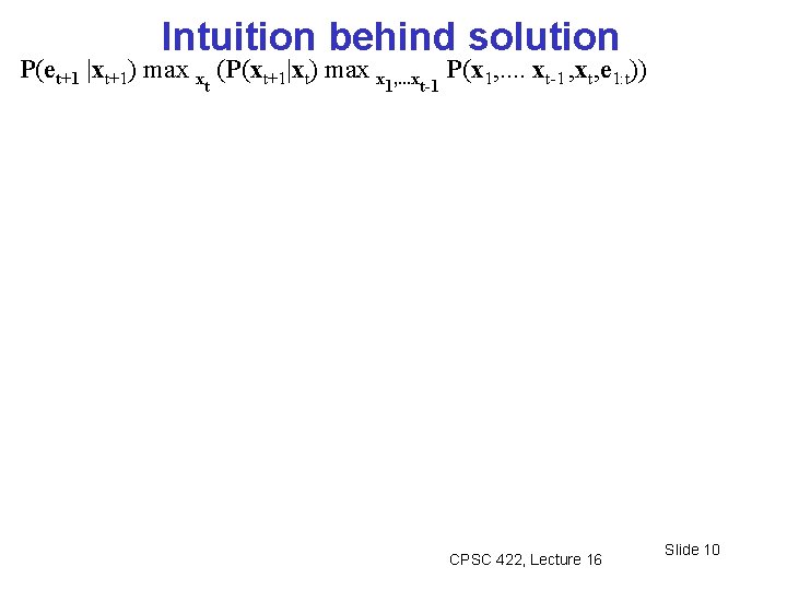
Intuition behind solution P(et+1 |xt+1) max x (P(xt+1|xt) max x t 1, . . . xt-1 P(x 1, . . xt-1 , xt, e 1: t)) CPSC 422, Lecture 16 Slide 10

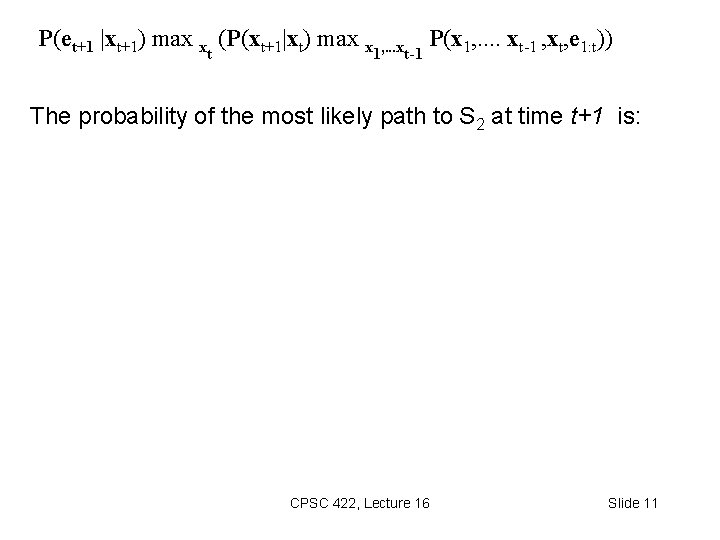
P(et+1 |xt+1) max x (P(xt+1|xt) max x t 1, . . . xt-1 P(x 1, . . xt-1 , xt, e 1: t)) The probability of the most likely path to S 2 at time t+1 is: CPSC 422, Lecture 16 Slide 11

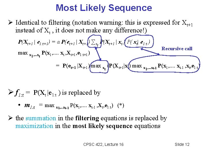
Most Likely Sequence Identical to filtering (notation warning: this is expressed for Xt+1 instead of Xt , it does not make any difference!) P(Xt+1 | e 1: t+1) = α P(et+1 | Xt+1) ∑xt P(Xt+1 | xt ) P( xt| e 1: t ) max x 1, . . . xt P(x 1, . . xt , Xt+1, e 1: t+1) = P(et+1 |Xt+1) max x (P(Xt+1|xt) max x t 1, . . . xt-1 Recursive call P(x 1, . . xt-1 , xt, e 1: t) f 1: t = P(Xt |e 1: t ) is replaced by • m 1: t = max x 1, . . . xt-1 P(x 1, . . xt-1 , Xt, e 1: t) (*) the summation in the filtering equations is replaced by maximization in the most likely sequence equations CPSC 422, Lecture 16 Slide 12

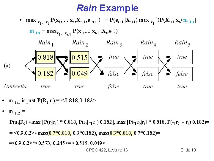
Rain Example • max x 1, . . . xt P(x 1, . . xt , Xt+1, e 1: t+1) = P(et+1 |Xt+1) max x [(P(Xt+1|xt) m 1: t] m 1: t = maxx t 1, . . . xt-1 P(x 1, . . xt-1 , Xt, e 1: t) 0. 818 0. 515 0. 182 0. 049 • m 1: 1 is just P(R 1|u) = <0. 818, 0. 182> • m 1: 2 = P(u 2|R 2) <max [P(r 2|r 1) * 0. 818, P(r 2| ┐r 1) 0. 182], max [P(┐r 2|r 1) * 0. 818, P(┐r 2| ┐r 1) 0. 182)= = <0. 9, 0. 2><max(0. 7*0. 818, 0. 3*0. 182), max(0. 3*0. 818, 0. 7*0. 182)= =<0. 9, 0. 2>*<0. 573, 0. 245>= <0. 515, 0. 049> CPSC 422, Lecture 16 Slide 13

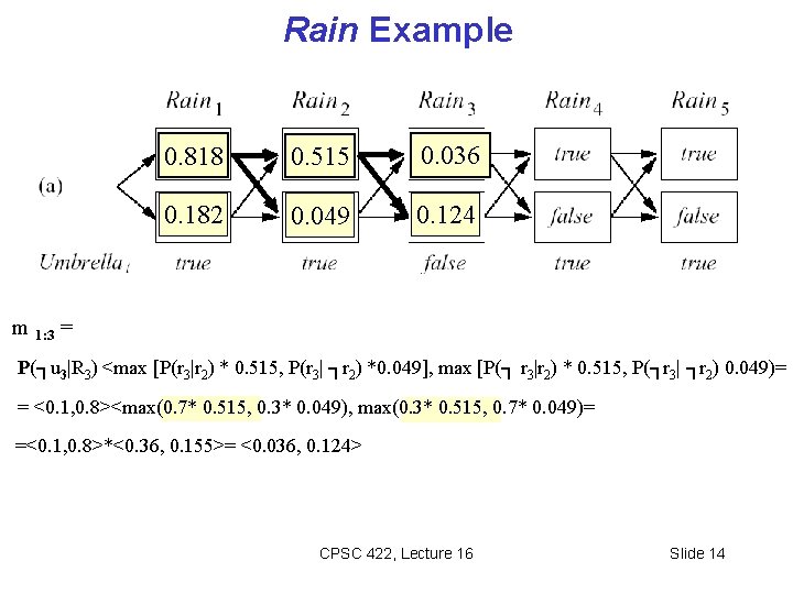
Rain Example 0. 818 0. 515 0. 036 0. 182 0. 049 0. 124 m 1: 3 = P(┐u 3|R 3) <max [P(r 3|r 2) * 0. 515, P(r 3| ┐r 2) *0. 049], max [P(┐ r 3|r 2) * 0. 515, P(┐r 3| ┐r 2) 0. 049)= = <0. 1, 0. 8><max(0. 7* 0. 515, 0. 3* 0. 049), max(0. 3* 0. 515, 0. 7* 0. 049)= =<0. 1, 0. 8>*<0. 36, 0. 155>= <0. 036, 0. 124> CPSC 422, Lecture 16 Slide 14

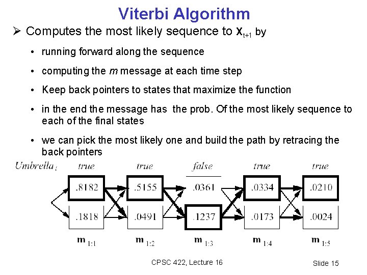
Viterbi Algorithm Computes the most likely sequence to Xt+1 by • running forward along the sequence • computing the m message at each time step • Keep back pointers to states that maximize the function • in the end the message has the prob. Of the most likely sequence to each of the final states • we can pick the most likely one and build the path by retracing the back pointers CPSC 422, Lecture 16 Slide 15

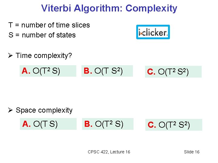
Viterbi Algorithm: Complexity T = number of time slices S = number of states Time complexity? A. O(T 2 S) B. O(T S 2) C. O(T 2 S 2) B. O(T 2 S) C. O(T 2 S 2) Space complexity A. O(T S) CPSC 422, Lecture 16 Slide 16

Lecture Overview Probabilistic temporal Inferences • Filtering • Prediction • Smoothing (forward-backward) • Most Likely Sequence of States (Viterbi) • Approx. Inference In Temporal Models (Particle Filtering) CPSC 422, Lecture 16 17

Limitations of Exact Algorithms • HMM has very large number of states • Our temporal model is a Dynamic Belief Network with several “state” variables Exact algorithms do not scale up What to do?

Approximate Inference Basic idea: • Draw N samples from known prob. distributions • Use those samples to estimate unknown prob. distributions Why sample? • Inference: getting N samples is faster than computing the right answer (e. g. with Filtering) CPSC 422, Lecture 11 19

Simple but Powerful Approach: Particle Filtering Idea from Exact Filtering: should be able to compute P(Xt+1 | e 1: t+1) from P( Xt | e 1: t ) “. . One slice from the previous slice…” Idea from Likelihood Weighting • Samples should be weighted by the probability of evidence given parents New Idea: run multiple samples simultaneously through the network CPSC 422, Lecture 11 20

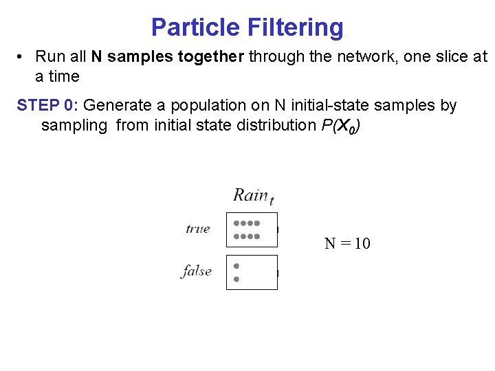
Particle Filtering • Run all N samples together through the network, one slice at a time STEP 0: Generate a population on N initial-state samples by sampling from initial state distribution P(X 0) N = 10

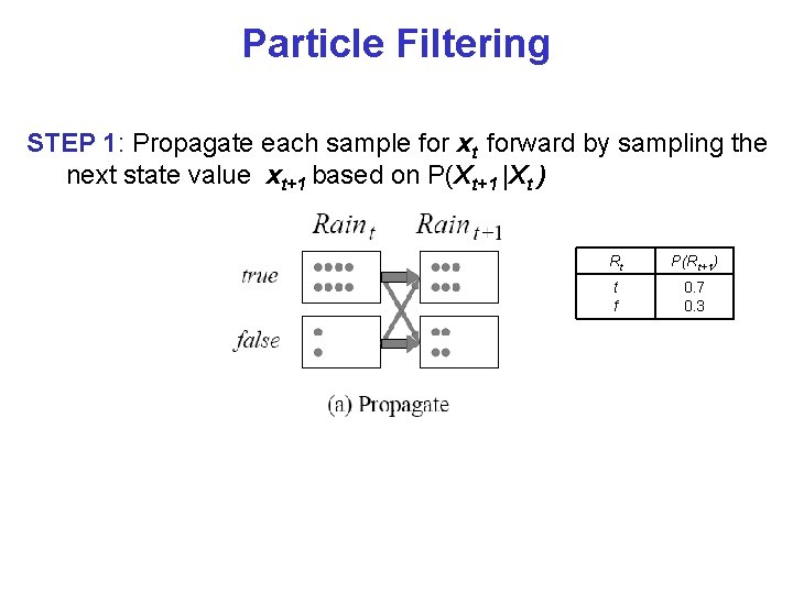
Particle Filtering STEP 1: Propagate each sample for xt forward by sampling the next state value xt+1 based on P(Xt+1 |Xt ) Rt P(Rt+1) t f 0. 7 0. 3

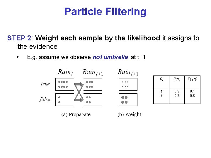
Particle Filtering STEP 2: Weight each sample by the likelihood it assigns to the evidence • E. g. assume we observe not umbrella at t+1 Rt P(ut) P(┐ut) t f 0. 9 0. 2 0. 1 0. 8

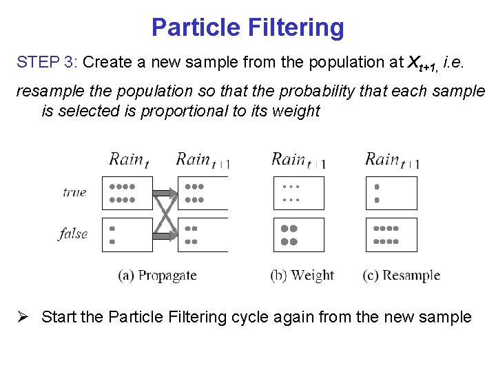
Particle Filtering STEP 3: Create a new sample from the population at Xt+1, i. e. resample the population so that the probability that each sample is selected is proportional to its weight Start the Particle Filtering cycle again from the new sample

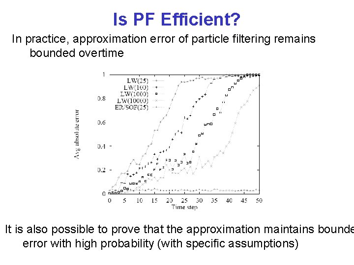
Is PF Efficient? In practice, approximation error of particle filtering remains bounded overtime It is also possible to prove that the approximation maintains bounde error with high probability (with specific assumptions)

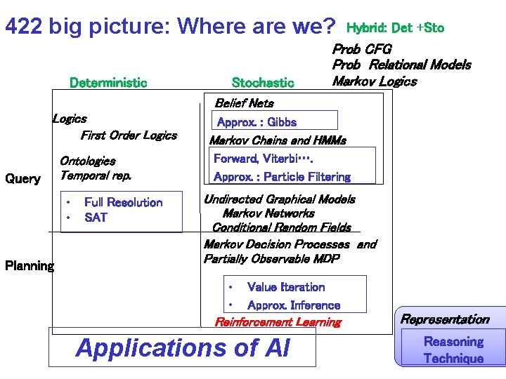
422 big picture: Where are we? Deterministic Logics First Order Logics Query Ontologies Temporal rep. • • Planning Full Resolution SAT Stochastic Belief Nets Hybrid: Det +Sto Prob CFG Prob Relational Models Markov Logics Approx. : Gibbs Markov Chains and HMMs Forward, Viterbi…. Approx. : Particle Filtering Undirected Graphical Models Markov Networks Conditional Random Fields Markov Decision Processes and Partially Observable MDP • Value Iteration • Approx. Inference Reinforcement Learning Applications of AI CPSC 322, Lecture 34 Representation Reasoning Technique Slide 26

Learning Goals for today’s class You can: • Describe the problem of finding the most likely sequence of states (given a sequence of observations), derive its solution (Viterbi algorithm) by manipulating probabilities and applying it to a temporal model • Describe and apply Particle Filtering for approx. inference in temporal models. CPSC 422, Lecture 16 Slide 27

TODO for Mon • Keep working on Assignment-2: RL, Approx. Inference in BN, Temporal Models - due Oct 21 Midterm Mon Oct 26 • Keep working on Assignment-2: RL, Approx. Inference in BN, Temporal Models - due Oct 21 CPSC 422, Lecture 16 Slide 28