Intelligent Systems AI2 Computer Science cpsc 422 Lecture

Intelligent Systems (AI-2) Computer Science cpsc 422, Lecture 18 Oct, 21, 2015 Slide Sources Raymond J. Mooney University of Texas at Austin D. Koller, Stanford CS - Probabilistic Graphical Models CPSC 422, Lecture 18 Slide 1

Lecture Overview Probabilistic Graphical models • Recap Markov Networks • Applications of Markov Networks • Inference in Markov Networks (Exact and Approx. ) • Conditional Random Fields CPSC 422, Lecture 17 2

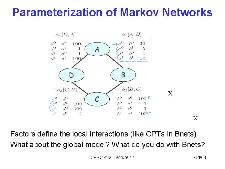
Parameterization of Markov Networks X X Factors define the local interactions (like CPTs in Bnets) What about the global model? What do you do with Bnets? CPSC 422, Lecture 17 Slide 3

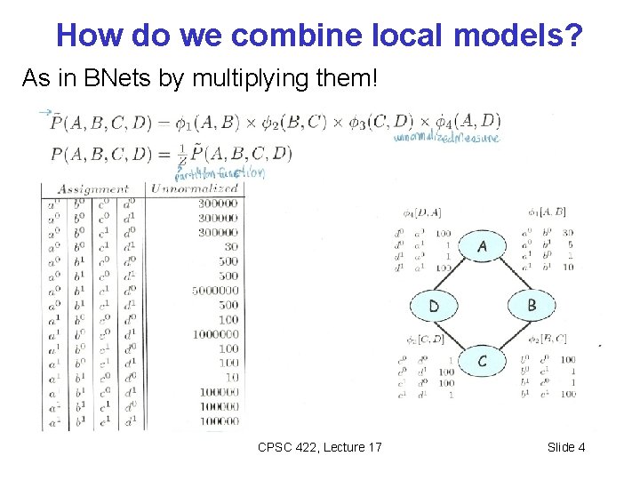
How do we combine local models? As in BNets by multiplying them! CPSC 422, Lecture 17 Slide 4

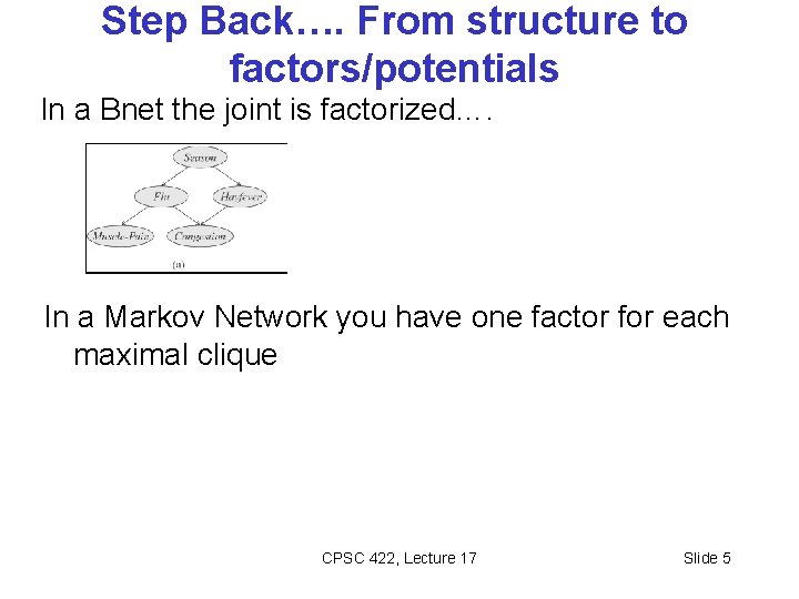
Step Back…. From structure to factors/potentials In a Bnet the joint is factorized…. In a Markov Network you have one factor for each maximal clique CPSC 422, Lecture 17 Slide 5

General definitions Two nodes in a Markov network are independent if and only if every path between them is cut off by evidence eg for A C So the markov blanket of a node is…? eg for C CPSC 422, Lecture 17 6

Lecture Overview Probabilistic Graphical models • Recap Markov Networks • Applications of Markov Networks • Inference in Markov Networks (Exact and Approx. ) • Conditional Random Fields CPSC 422, Lecture 17 7

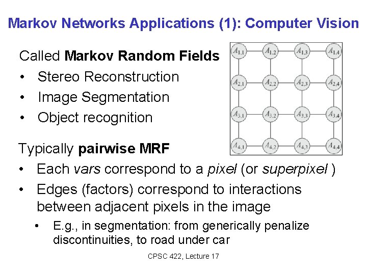
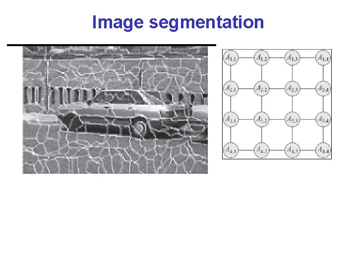
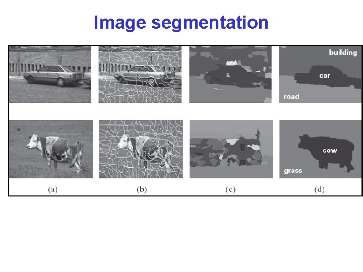
Markov Networks Applications (1): Computer Vision Called Markov Random Fields • Stereo Reconstruction • Image Segmentation • Object recognition Typically pairwise MRF • Each vars correspond to a pixel (or superpixel ) • Edges (factors) correspond to interactions between adjacent pixels in the image • E. g. , in segmentation: from generically penalize discontinuities, to road under car CPSC 422, Lecture 17 8

Image segmentation CPSC 422, Lecture 17 9

Image segmentation CPSC 422, Lecture 17 10

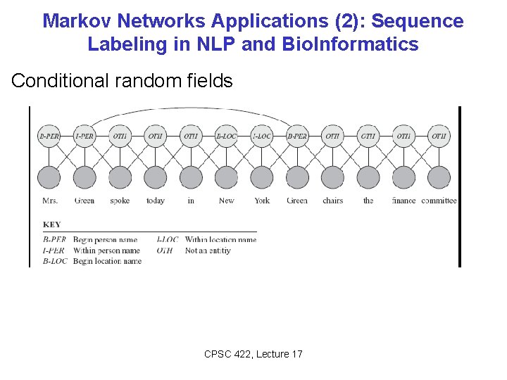
Markov Networks Applications (2): Sequence Labeling in NLP and Bio. Informatics Conditional random fields CPSC 422, Lecture 17 11

Lecture Overview Probabilistic Graphical models • Recap Markov Networks • Applications of Markov Networks • Inference in Markov Networks (Exact and Approx. ) • Conditional Random Fields CPSC 422, Lecture 17 12

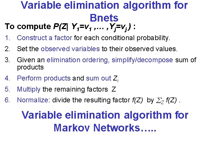
Variable elimination algorithm for Bnets To compute P(Z| Y 1=v 1 , … , Yj=vj ) : 1. Construct a factor for each conditional probability. 2. Set the observed variables to their observed values. 3. Given an elimination ordering, simplify/decompose sum of products 4. Perform products and sum out Zi 5. Multiply the remaining factors Z 6. Normalize: divide the resulting factor f(Z) by Z f(Z). Variable elimination algorithm for Markov Networks…. . CPSC 422, Lecture 17 Slide 13

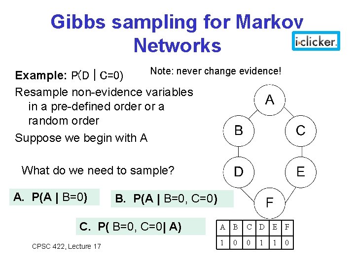
Gibbs sampling for Markov Networks Note: never change evidence! Example: P(D | C=0) Resample non-evidence variables in a pre-defined order or a random order Suppose we begin with A What do we need to sample? A. P(A | B=0) B. P(A | B=0, C=0) C. P( B=0, C=0| A) CPSC 422, Lecture 17 A B C D E F 1 0 0 1 1 0 14

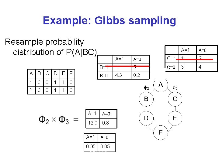
Example: Gibbs sampling Resample probability distribution of P(A|BC) A B C D E F 1 0 0 1 1 0 ? 0 0 1 1 0 A=1 A=0 C=1 1 2 B=1 1 5 C=0 3 4 B=0 4. 3 0. 2 A=0 12. 9 0. 8 Normalized result = A=1 A=0 0. 95 0. 05 CPSC 422, Lecture 17 15

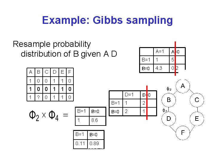
Example: Gibbs sampling Resample probability distribution of B given A D A B C D E F 1 0 0 1 1 A=0 B=1 1 5 B=0 4. 3 0. 2 0 1 0 0 1 1 0 1 ? 0 1 1 D=0 B=1 1 2 B=0 2 1 0 Normalized result = B=1 B=0 1 8. 6 B=1 B=0 0. 11 0. 89 CPSC 422, Lecture 17 16

Lecture Overview Probabilistic Graphical models • Recap Markov Networks • Applications of Markov Networks • Inference in Markov Networks (Exact and Approx. ) • Conditional Random Fields CPSC 422, Lecture 17 17

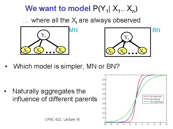
We want to model P(Y 1| X 1. . Xn) … where all the Xi are always observed MN Y 1 X 2 …X BN Y 1 n X 1 X 2 …X n • Which model is simpler, MN or BN? • Naturally aggregates the influence of different parents CPSC 422, Lecture 18 Slide 18

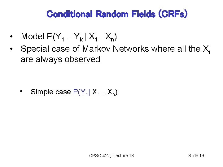
Conditional Random Fields (CRFs) • Model P(Y 1. . Yk | X 1. . Xn) • Special case of Markov Networks where all the Xi are always observed • Simple case P(Y 1| X 1…Xn) CPSC 422, Lecture 18 Slide 19

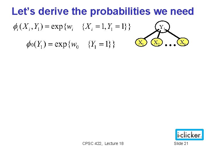
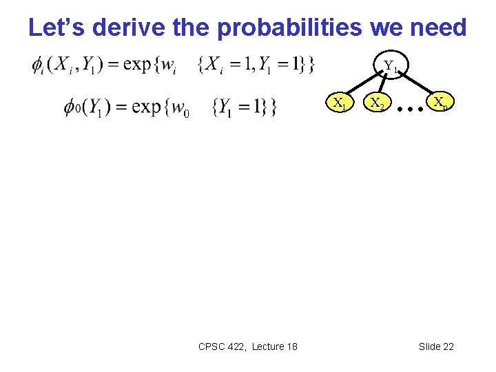
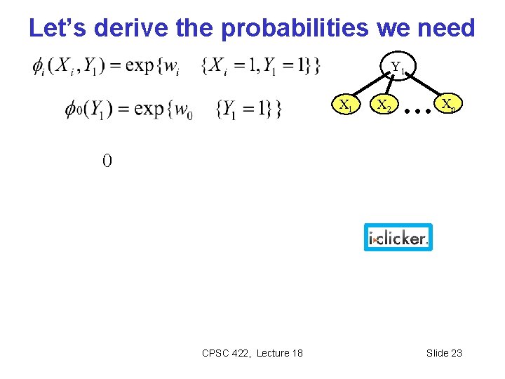
What are the Parameters? CPSC 422, Lecture 18 Slide 20

Let’s derive the probabilities we need Y 1 X 1 CPSC 422, Lecture 18 X 2 …X n Slide 21

Let’s derive the probabilities we need Y 1 X 1 CPSC 422, Lecture 18 X 2 …X n Slide 22

Let’s derive the probabilities we need Y 1 X 2 …X n 0 CPSC 422, Lecture 18 Slide 23

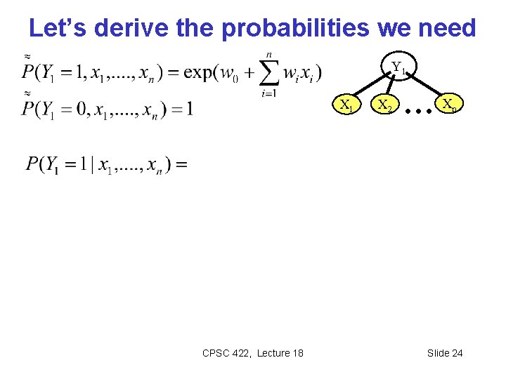
Let’s derive the probabilities we need Y 1 X 1 CPSC 422, Lecture 18 X 2 …X n Slide 24

Let’s derive the probabilities we need Y 1 X 1 CPSC 422, Lecture 18 X 2 …X n Slide 25

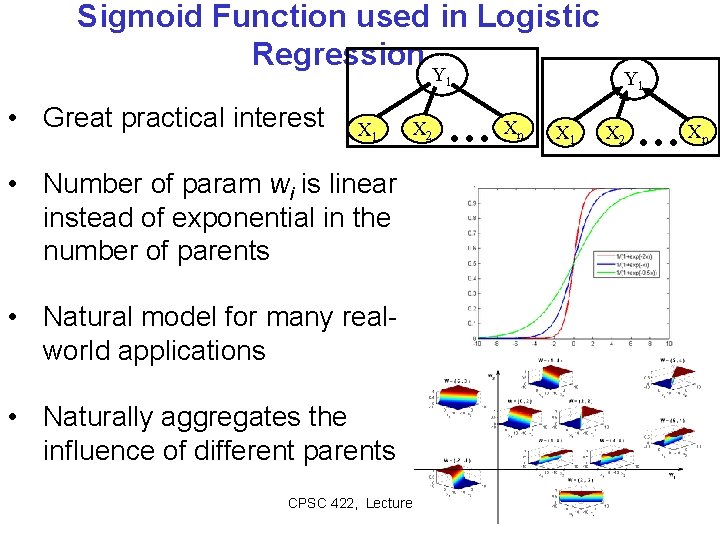
Sigmoid Function used in Logistic Regression Y 1 • Great practical interest X 1 X 2 …X n X 1 Y 1 X 2 …X • Number of param wi is linear instead of exponential in the number of parents • Natural model for many realworld applications • Naturally aggregates the influence of different parents CPSC 422, Lecture 18 Slide 26 n

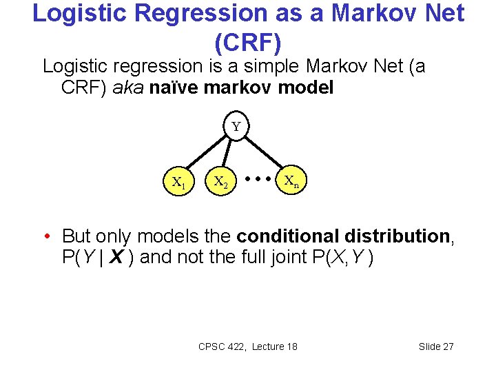
Logistic Regression as a Markov Net (CRF) Logistic regression is a simple Markov Net (a CRF) aka naïve markov model Y X 1 X 2 … Xn • But only models the conditional distribution, P(Y | X ) and not the full joint P(X, Y ) CPSC 422, Lecture 18 Slide 27

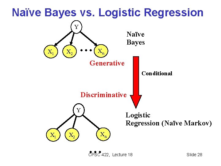
Naïve Bayes vs. Logistic Regression Y X 1 X 2 … Naïve Bayes Xn Generative Conditional Discriminative Y X 1 X 2 Logistic Regression (Naïve Markov) Xn … CPSC 422, Lecture 18 Slide 28

Learning Goals for today’s class You can: • Perform Exact and Approx. Inference in Markov Networks • Describe a few applications of Markov Networks • Describe a natural parameterization for a Naïve Markov model (which is a simple CRF) • Derive how P(Y|X) can be computed for a Naïve Markov model • Explain the discriminative vs. generative distinction and its implications CPSC 422, Lecture 18 Slide 29

Next class Fri To Do Linear-chain CRFs Revise generative temporal models (HMM) Midterm, Mon, Oct 26, we will start at 9 am sharp How to prepare…. • • Work on practice material posted on Connect Learning Goals (look at the end of the slides for each lecture – or complete list on Connect) • Go to Office Hours (Ted is offering and extra slot on Fri check Piazza • Revise all the clicker questions and practice exercises CPSC 422, Lecture 18 Slide 30

Midterm, Mon, Oct 26, we will start at 9 am sharp How to prepare…. • Keep Working on assignment-2 ! • Go to Office Hours x • Learning Goals (look at the end of the slides for each lecture – will post complete list) • Revise all the clicker questions and practice exercises • Will post more practice material today CPSC 422, Lecture 17 Slide 31

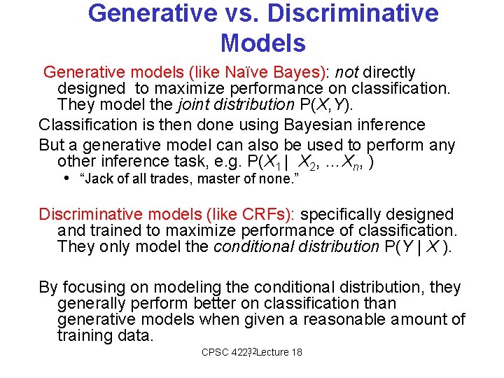
Generative vs. Discriminative Models Generative models (like Naïve Bayes): not directly designed to maximize performance on classification. They model the joint distribution P(X, Y). Classification is then done using Bayesian inference But a generative model can also be used to perform any other inference task, e. g. P(X 1 | X 2, …Xn, ) • “Jack of all trades, master of none. ” Discriminative models (like CRFs): specifically designed and trained to maximize performance of classification. They only model the conditional distribution P(Y | X ). By focusing on modeling the conditional distribution, they generally perform better on classification than generative models when given a reasonable amount of training data. CPSC 422, 32 Lecture 18

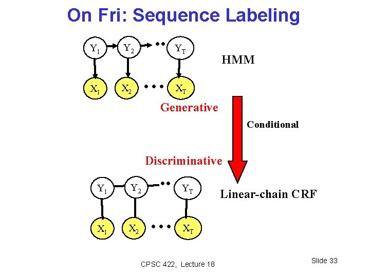
On Fri: Sequence Labeling Y 1 Y 2 . . X 1 X 2 … YT HMM XT Generative Conditional Discriminative Y 1 Y 2 X 1 X 2 . . … YT Linear-chain CRF XT CPSC 422, Lecture 18 Slide 33

Lecture Overview • Indicator function • P(X, Y) vs. P(X|Y) and Naïve Bayes • Model P(Y|X) explicitly with Markov Networks • Parameterization • Inference • Generative vs. Discriminative models CPSC 422, Lecture 18 34

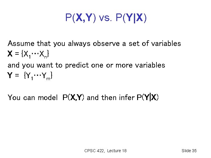
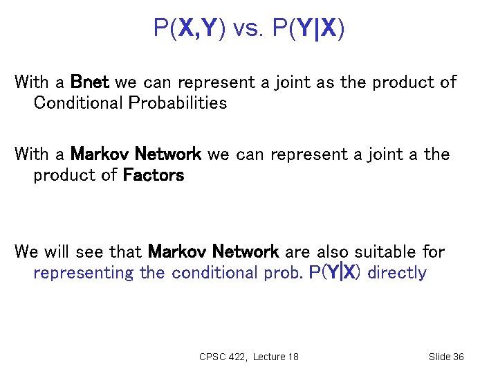
P(X, Y) vs. P(Y|X) Assume that you always observe a set of variables X = {X 1…Xn} and you want to predict one or more variables Y = {Y 1…Ym} You can model P(X, Y) and then infer P(Y|X) CPSC 422, Lecture 18 Slide 35

P(X, Y) vs. P(Y|X) With a Bnet we can represent a joint as the product of Conditional Probabilities With a Markov Network we can represent a joint a the product of Factors We will see that Markov Network are also suitable for representing the conditional prob. P(Y|X) directly CPSC 422, Lecture 18 Slide 36

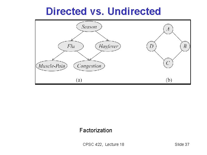
Directed vs. Undirected Factorization CPSC 422, Lecture 18 Slide 37

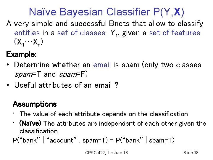
Naïve Bayesian Classifier P(Y, X) A very simple and successful Bnets that allow to classify entities in a set of classes Y 1, given a set of features (X 1…Xn) Example: • Determine whether an email is spam (only two classes spam=T and spam=F) • Useful attributes of an email ? Assumptions • The value of each attribute depends on the classification • (Naïve) The attributes are independent of each other given the classification P(“bank” | “account” , spam=T) = P(“bank” | spam=T) CPSC 422, Lecture 18 Slide 38

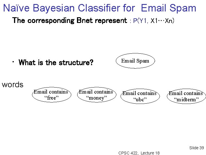
Naïve Bayesian Classifier for Email Spam The corresponding Bnet represent : P(Y 1, X 1…Xn) • What is the structure? words Email contains “free” Email contains “money” Email Spam Email contains “ubc” Email contains “midterm” Slide 39 CPSC 422, Lecture 18

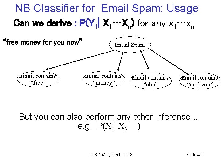
NB Classifier for Email Spam: Usage Can we derive : P(Y 1| X 1…Xn) for any x 1…xn “free money for you now” Email contains “free” Email Spam Email contains “money” Email contains “ubc” Email contains “midterm” But you can also perform any other inference… e. g. , P(X 1| X 3 ) CPSC 422, Lecture 18 Slide 40

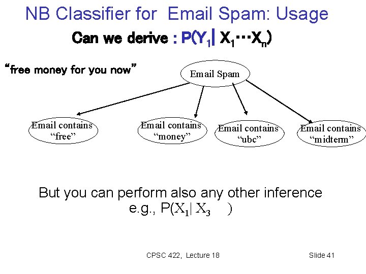
NB Classifier for Email Spam: Usage Can we derive : P(Y 1| X 1…Xn) “free money for you now” Email contains “free” Email Spam Email contains “money” Email contains “ubc” Email contains “midterm” But you can perform also any other inference e. g. , P(X 1| X 3 ) CPSC 422, Lecture 18 Slide 41

CPSC 422, Lecture 18 Slide 42