Integration Copyright Cengage Learning All rights reserved 4

Integration Copyright © Cengage Learning. All rights reserved.

4. 5 Integration by Substitution Copyright © Cengage Learning. All rights reserved.

Objectives n Use pattern recognition to find an indefinite integral. n Use a change of variables to find an indefinite integral. n Use the General Power Rule for Integration to find an indefinite integral. n Use a change of variables to evaluate a definite integral. n Evaluate a definite integral involving an even or odd function. 3

Pattern Recognition 4

Pattern Recognition In this section you will study techniques for integrating composite functions. The discussion is split into two parts—pattern recognition and change of variables. Both techniques involve a u-substitution. With pattern recognition, you perform the substitution mentally, and with change of variables, you write the substitution steps. The role of substitution in integration is comparable to the role of the Chain Rule in differentiation. 5

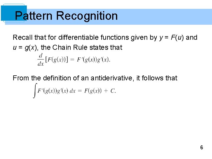
Pattern Recognition Recall that for differentiable functions given by y = F(u) and u = g(x), the Chain Rule states that From the definition of an antiderivative, it follows that 6

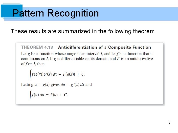
Pattern Recognition These results are summarized in the following theorem. 7

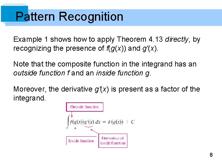
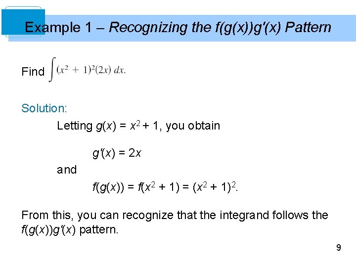
Pattern Recognition Example 1 shows how to apply Theorem 4. 13 directly, by recognizing the presence of f(g(x)) and g'(x). Note that the composite function in the integrand has an outside function f and an inside function g. Moreover, the derivative g'(x) is present as a factor of the integrand. 8

Example 1 – Recognizing the f(g(x))g'(x) Pattern Find Solution: Letting g(x) = x 2 + 1, you obtain g'(x) = 2 x and f(g(x)) = f(x 2 + 1) = (x 2 + 1)2. From this, you can recognize that the integrand follows the f(g(x))g'(x) pattern. 9

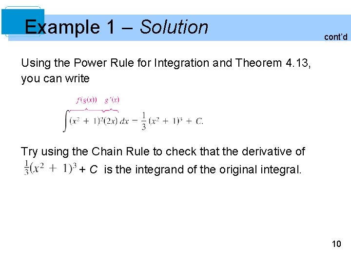
Example 1 – Solution cont’d Using the Power Rule for Integration and Theorem 4. 13, you can write Try using the Chain Rule to check that the derivative of + C is the integrand of the original integral. 10

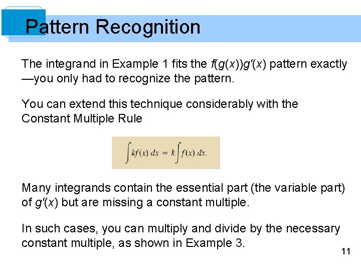
Pattern Recognition The integrand in Example 1 fits the f(g(x))g'(x) pattern exactly —you only had to recognize the pattern. You can extend this technique considerably with the Constant Multiple Rule Many integrands contain the essential part (the variable part) of g'(x) but are missing a constant multiple. In such cases, you can multiply and divide by the necessary constant multiple, as shown in Example 3. 11

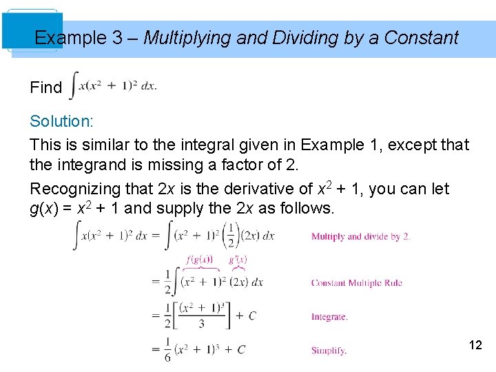
Example 3 – Multiplying and Dividing by a Constant Find Solution: This is similar to the integral given in Example 1, except that the integrand is missing a factor of 2. Recognizing that 2 x is the derivative of x 2 + 1, you can let g(x) = x 2 + 1 and supply the 2 x as follows. 12

Change of Variables 13

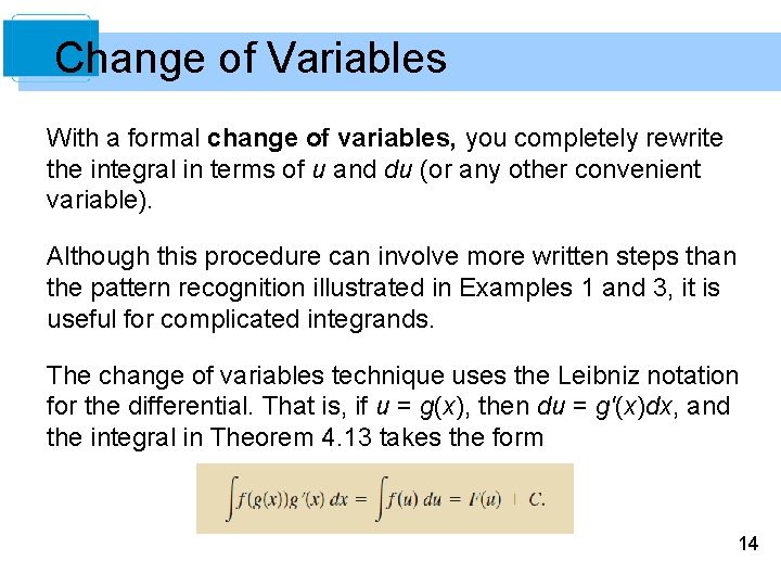
Change of Variables With a formal change of variables, you completely rewrite the integral in terms of u and du (or any other convenient variable). Although this procedure can involve more written steps than the pattern recognition illustrated in Examples 1 and 3, it is useful for complicated integrands. The change of variables technique uses the Leibniz notation for the differential. That is, if u = g(x), then du = g'(x)dx, and the integral in Theorem 4. 13 takes the form 14

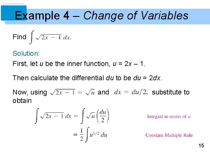
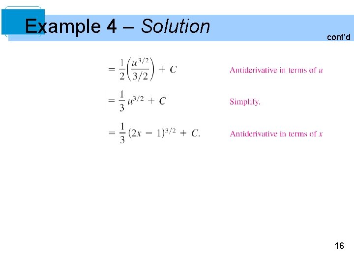
Example 4 – Change of Variables Find Solution: First, let u be the inner function, u = 2 x – 1. Then calculate the differential du to be du = 2 dx. Now, using obtain and substitute to 15

Example 4 – Solution cont’d 16

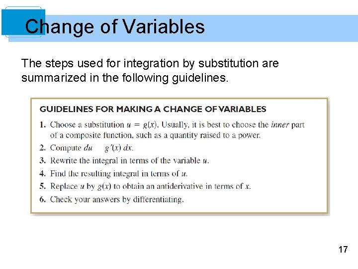
Change of Variables The steps used for integration by substitution are summarized in the following guidelines. 17

The General Power Rule for Integration 18

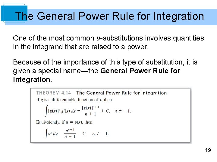
The General Power Rule for Integration One of the most common u-substitutions involves quantities in the integrand that are raised to a power. Because of the importance of this type of substitution, it is given a special name—the General Power Rule for Integration. 19

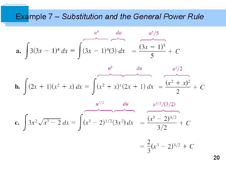
Example 7 – Substitution and the General Power Rule 20

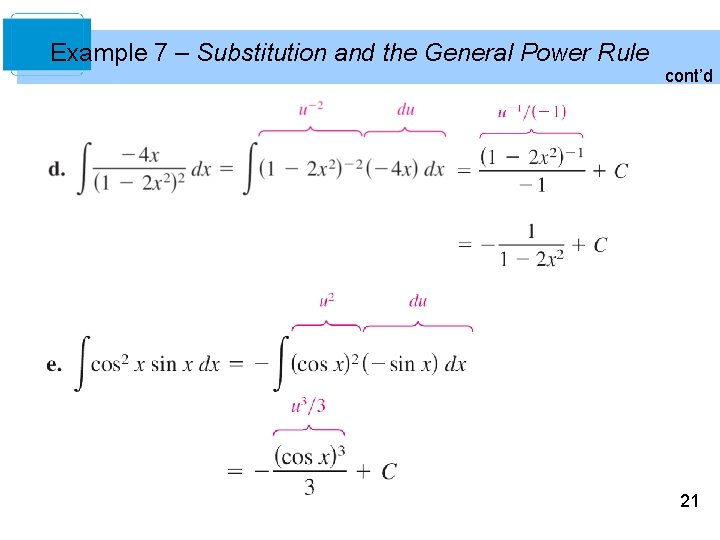
Example 7 – Substitution and the General Power Rule cont’d 21

Change of Variables for Definite Integrals 22

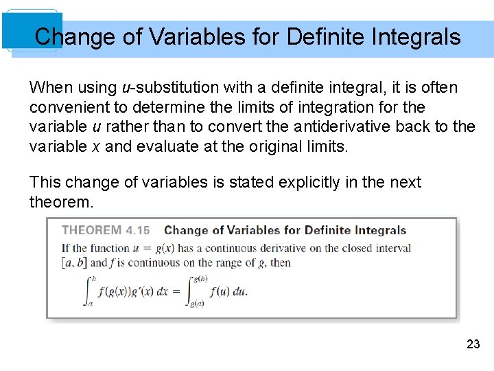
Change of Variables for Definite Integrals When using u-substitution with a definite integral, it is often convenient to determine the limits of integration for the variable u rather than to convert the antiderivative back to the variable x and evaluate at the original limits. This change of variables is stated explicitly in the next theorem. 23

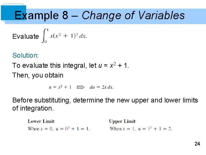
Example 8 – Change of Variables Evaluate Solution: To evaluate this integral, let u = x 2 + 1. Then, you obtain Before substituting, determine the new upper and lower limits of integration. 24

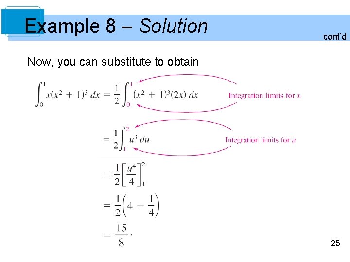
Example 8 – Solution cont’d Now, you can substitute to obtain 25

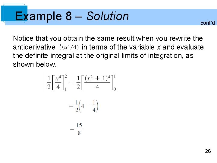
Example 8 – Solution cont’d Notice that you obtain the same result when you rewrite the antiderivative in terms of the variable x and evaluate the definite integral at the original limits of integration, as shown below. 26

Integration of Even and Odd Functions 27

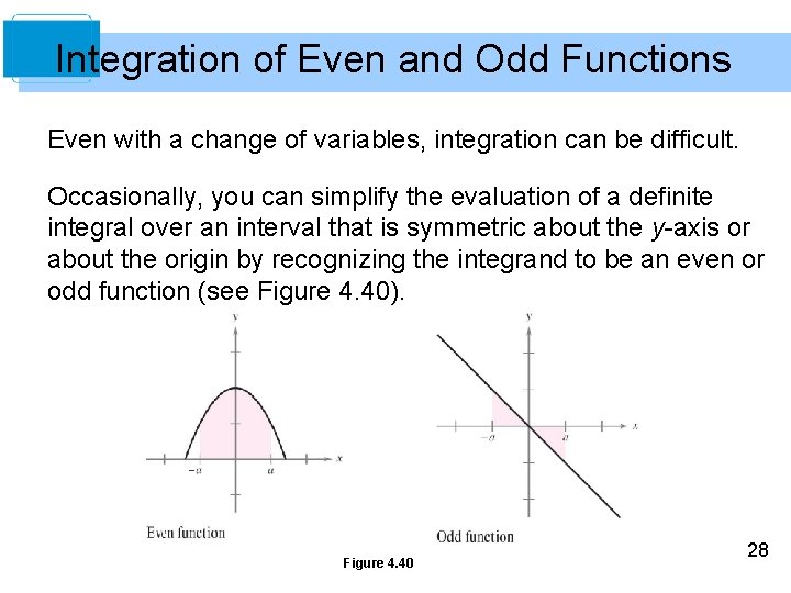
Integration of Even and Odd Functions Even with a change of variables, integration can be difficult. Occasionally, you can simplify the evaluation of a definite integral over an interval that is symmetric about the y-axis or about the origin by recognizing the integrand to be an even or odd function (see Figure 4. 40). Figure 4. 40 28

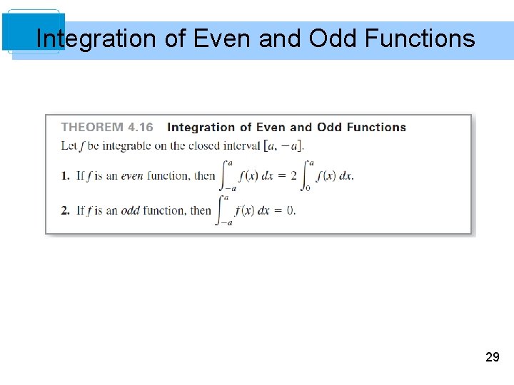
Integration of Even and Odd Functions 29

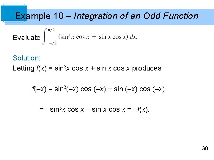
Example 10 – Integration of an Odd Function Evaluate Solution: Letting f(x) = sin 3 x cos x + sin x cos x produces f(–x) = sin 3(–x) cos (–x) + sin (–x) cos (–x) = –sin 3 x cos x – sin x cos x = –f(x). 30

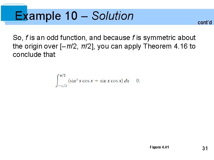
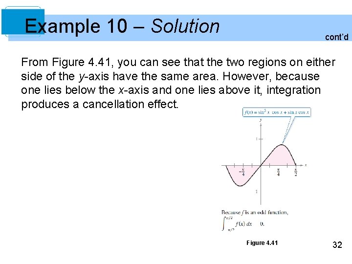
Example 10 – Solution cont’d So, f is an odd function, and because f is symmetric about the origin over [–π/2, π/2], you can apply Theorem 4. 16 to conclude that Figure 4. 41 31

Example 10 – Solution cont’d From Figure 4. 41, you can see that the two regions on either side of the y-axis have the same area. However, because one lies below the x-axis and one lies above it, integration produces a cancellation effect. Figure 4. 41 32