INFSY 540 1 Information Resources in Management Lesson

INFSY 540. 1 Information Resources in Management Lesson #4 Chapters 8 Models and Decision Support Copyright © 1998 by Jerry Post 1

Information Systems & Technology An information system (IS) is an arrangement of people, data, processes, communications, and information technology that interact to support and improve day-to-day operations in a business as well as support the problem-solving and decision making needs of management and users. Information technology is a contemporary term that describes the combination of computer technology (hardware and software) with telecommunications technology (data, image, and voice networks). A practical way of making data useful. 2

What is an information system? 3

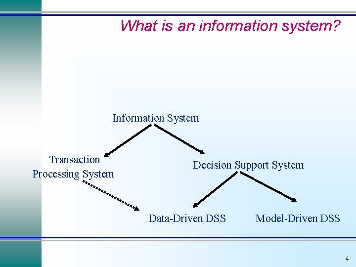
What is an information system? Information System Transaction Processing System Decision Support System Data-Driven DSS Model-Driven DSS 4

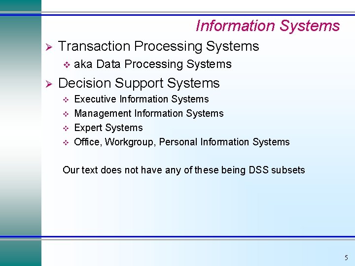
Information Systems Ø Transaction Processing Systems v Ø aka Data Processing Systems Decision Support Systems v v Executive Information Systems Management Information Systems Expert Systems Office, Workgroup, Personal Information Systems Our text does not have any of these being DSS subsets 5

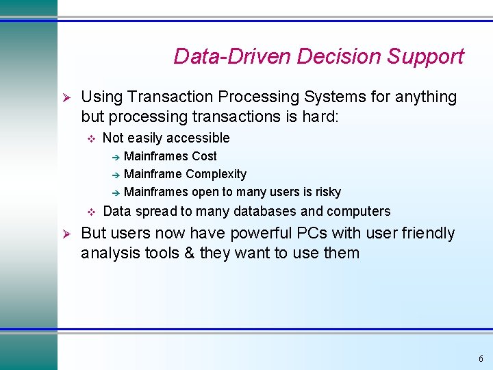
Data-Driven Decision Support Ø Using Transaction Processing Systems for anything but processing transactions is hard: v Not easily accessible Mainframes Cost è Mainframe Complexity è Mainframes open to many users is risky è v Ø Data spread to many databases and computers But users now have powerful PCs with user friendly analysis tools & they want to use them 6

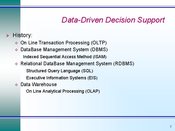
Data-Driven Decision Support Ø History: v v On Line Transaction Processing (OLTP) Data. Base Management System (DBMS) Indexed Sequential Access Method (ISAM) v Relational Data. Base Management System (RDBMS) Structured Query Language (SQL) Executive Information Systems (EIS) v Data Warehouse On Line Analytical Processing (OLAP) 7

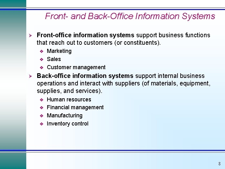
Front- and Back-Office Information Systems Ø Front-office information systems support business functions that reach out to customers (or constituents). v v v Ø Marketing Sales Customer management Back-office information systems support internal business operations and interact with suppliers (of materials, equipment, supplies, and services). v v Human resources Financial management Manufacturing Inventory control 8

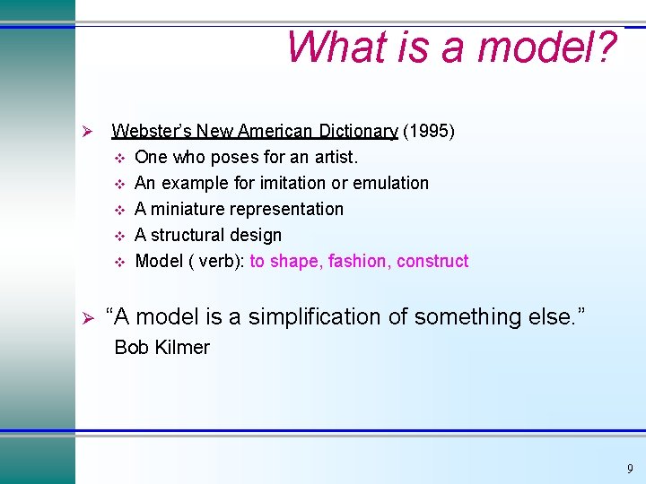
What is a model? Ø Ø Webster’s New American Dictionary (1995) v One who poses for an artist. v An example for imitation or emulation v A miniature representation v A structural design v Model ( verb): to shape, fashion, construct “A model is a simplification of something else. ” Bob Kilmer 9

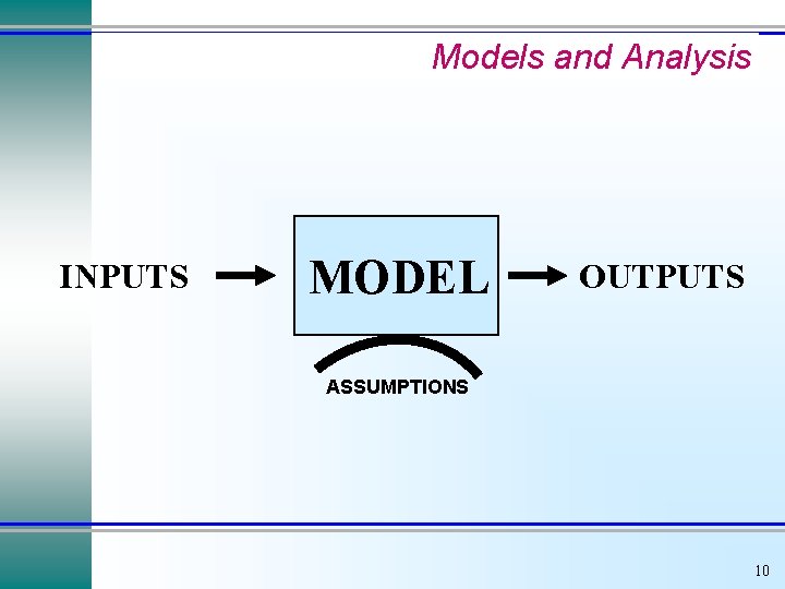
Models and Analysis INPUTS MODEL OUTPUTS ASSUMPTIONS 10

Assumptions and Conclusions The aviation instructor had just delivered a lecture on the use of parachutes. “And if it doesn’t open? ” someone asked. “If it doesn’t open? ” replied the instructor, “Well, . . . that is what’s known as jumping to a conclusion. ” 11

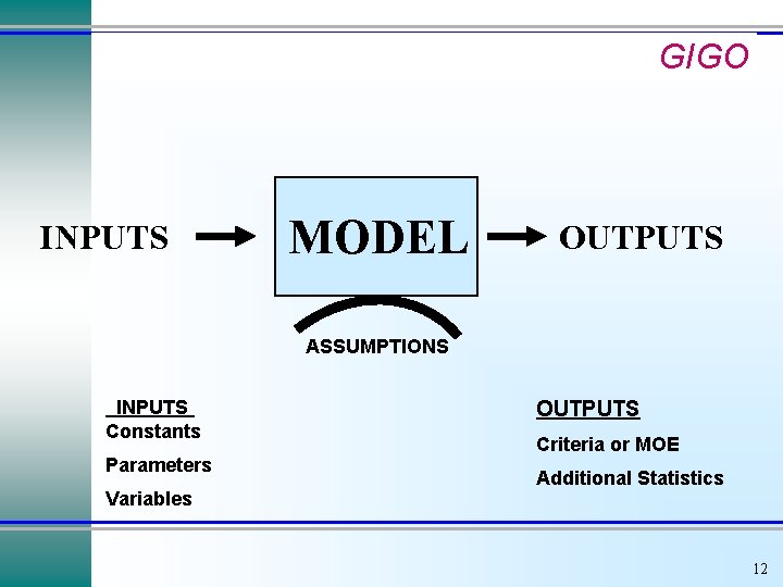
GIGO INPUTS MODEL OUTPUTS ASSUMPTIONS INPUTS Constants Parameters Variables OUTPUTS Criteria or MOE Additional Statistics 12

Types of Models Ø Ø Ø Mental Symbolic Mathematical Computer Physical 13

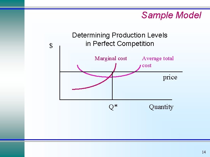
Sample Model $ Determining Production Levels in Perfect Competition Marginal cost Average total cost price Q* Quantity 14

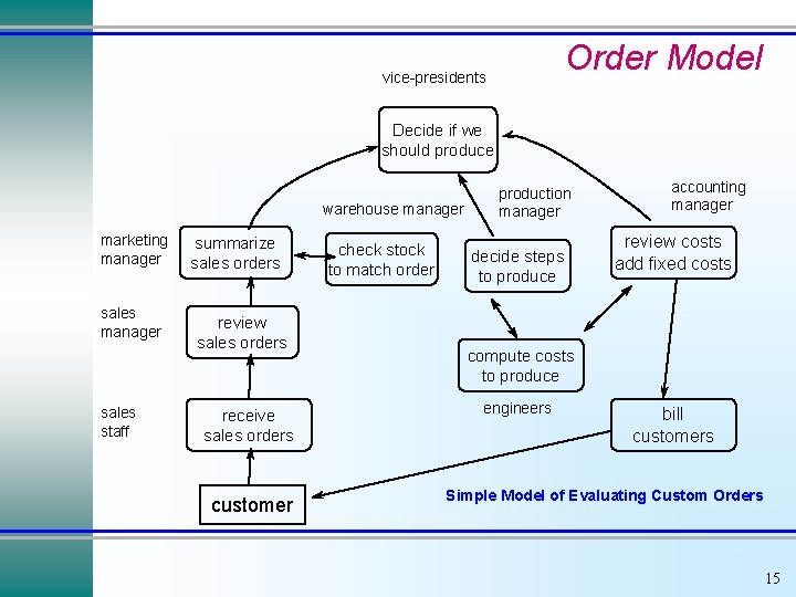
Order Model vice-presidents Decide if we should produce warehouse manager marketing manager sales staff summarize sales orders review sales orders receive sales orders customer check stock to match order production manager decide steps to produce accounting manager review costs add fixed costs compute costs to produce engineers bill customers Simple Model of Evaluating Custom Orders 15

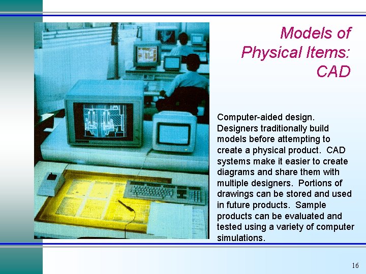
Models of Physical Items: CAD Computer-aided design. Designers traditionally build models before attempting to create a physical product. CAD systems make it easier to create diagrams and share them with multiple designers. Portions of drawings can be stored and used in future products. Sample products can be evaluated and tested using a variety of computer simulations. 16

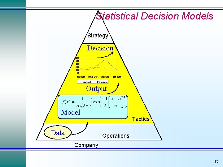
Statistical Decision Models Strategy Decision Output Model Data Tactics Operations Company 17

File: C 08 Fig 08. xls Why Build Models? Ø Ø Ø Understand the Process Prediction Optimization Simulation To conduct "What If" analysis Dangers 18

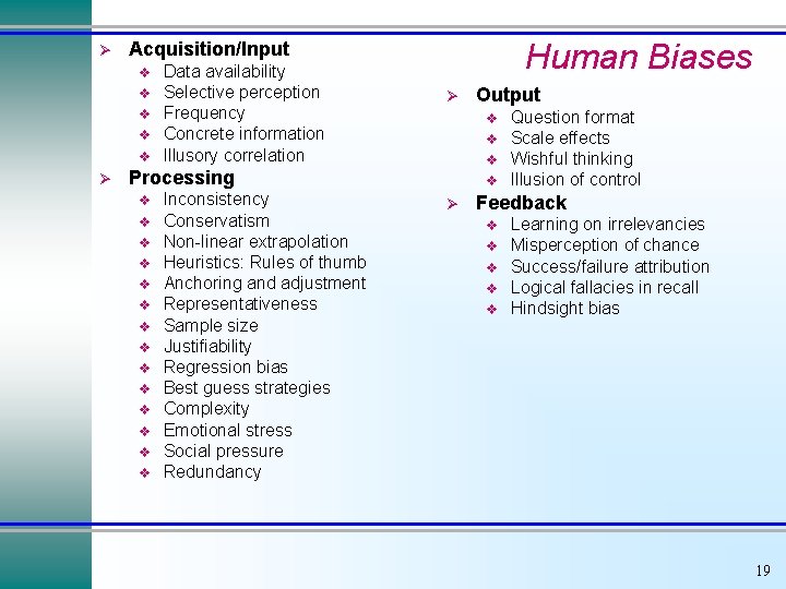
Ø v v v Ø Human Biases Acquisition/Input Data availability Selective perception Frequency Concrete information Illusory correlation Ø v v v Processing v v v v Inconsistency Conservatism Non-linear extrapolation Heuristics: Rules of thumb Anchoring and adjustment Representativeness Sample size Justifiability Regression bias Best guess strategies Complexity Emotional stress Social pressure Redundancy Output v Ø Question format Scale effects Wishful thinking Illusion of control Feedback v v v Learning on irrelevancies Misperception of chance Success/failure attribution Logical fallacies in recall Hindsight bias 19

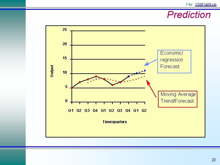
File: C 08 Fig 09. xls Prediction 25 20 Economic/ regression Forecast Output 15 10 5 Moving Average Trend/Forecast 0 Q 1 Q 2 Q 3 Q 4 Q 1 Q 2 Time/quarters 20

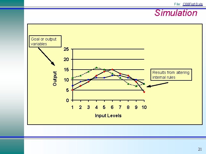
File: C 08 Fig 10. xls Simulation Goal or output variables 25 Output 20 15 Results from altering internal rules 10 5 0 1 2 3 4 5 6 7 8 9 10 Input Levels 21

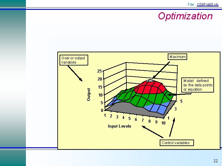
File: C 08 Fig 08. xls Optimization Maximum Goal or output variables 25 Output 20 Model: defined by the data points or equation 15 10 5 5 3 0 1 2 3 4 5 Input Levels 6 7 8 9 10 1 Control variables 22

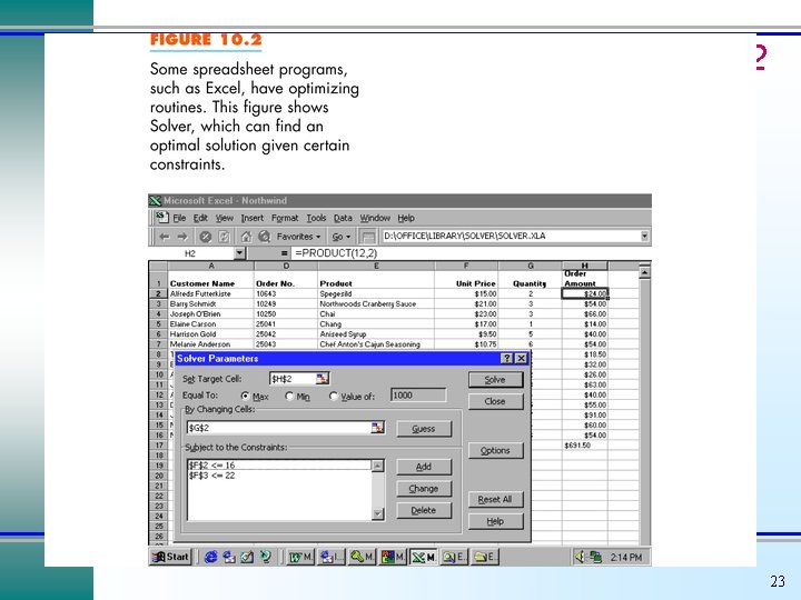
Figure 10. 2 23

Simulation Ø Webster’s New American Dictionary (1995) v An object that is not genuine v The imitation by one system or process of the way in which another system or process works. v Simulate (verb): imitate, create the effect or appearance of Ø Handbook of Systems Analysis (1985), E. S. Quade v “The process of representing item by item and step by step the essential features of whatever it is we are interested in. ” 24

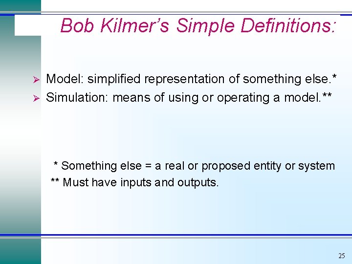
Bob Kilmer’s Simple Definitions: Ø Ø Model: simplified representation of something else. * Simulation: means of using or operating a model. ** * Something else = a real or proposed entity or system ** Must have inputs and outputs. 25

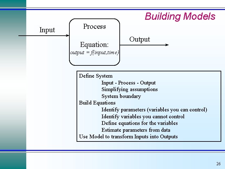
Building Models Input Process Equation: Output output = f(input, time) Define System Input - Process - Output Simplifying assumptions System boundary Build Equations Identify parameters (variables you can control) Identify variables you cannot control Define equations for the variables Estimate parameters from data Use Model to transform Inputs into Outputs 26

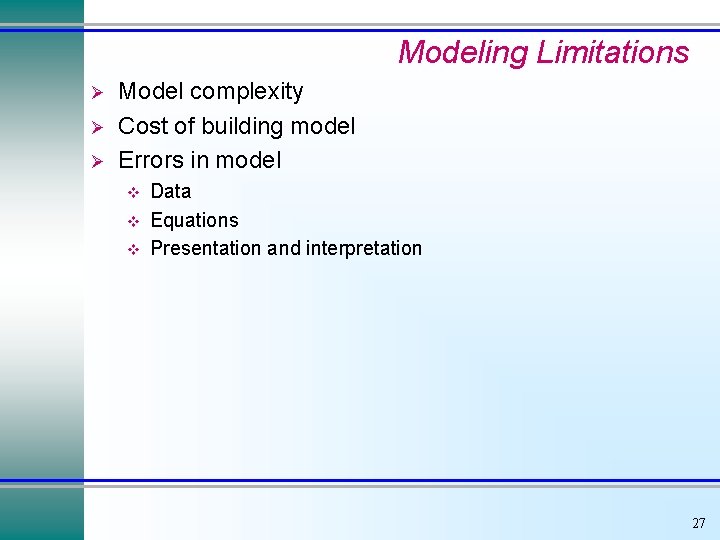
Modeling Limitations Ø Ø Ø Model complexity Cost of building model Errors in model v v v Data Equations Presentation and interpretation 27

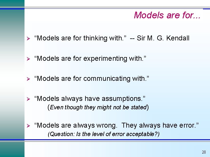
Models are for. . . Ø “Models are for thinking with. ” -- Sir M. G. Kendall Ø “Models are for experimenting with. ” Ø “Models are for communicating with. ” Ø “Models always have assumptions. ” (Even though they might not be stated) Ø “Models are always wrong. They always have error. ” (Question: Is the level of error acceptable? ) 28

EOQ Model 29

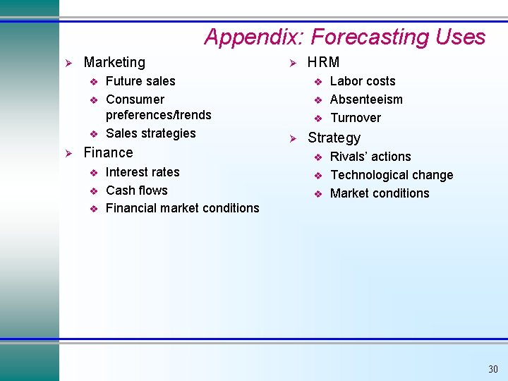
Appendix: Forecasting Uses Ø Marketing v v v Ø Future sales Consumer preferences/trends Sales strategies Finance v v v Interest rates Cash flows Financial market conditions Ø HRM v v v Ø Labor costs Absenteeism Turnover Strategy v v v Rivals’ actions Technological change Market conditions 30

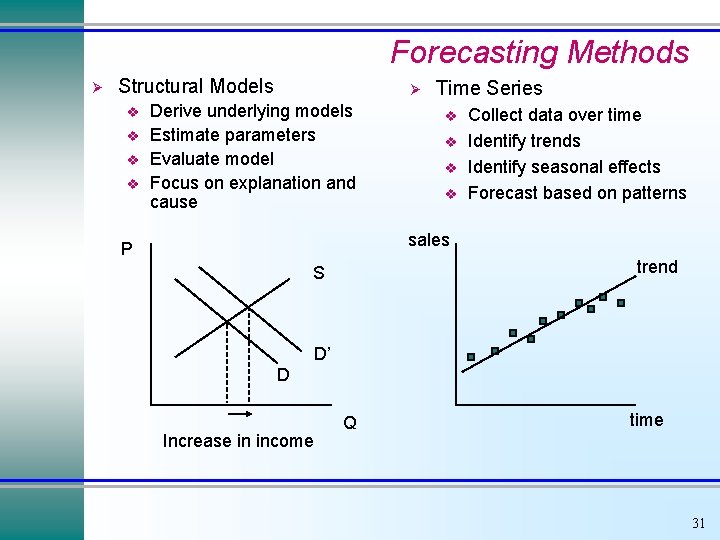
Forecasting Methods Ø Structural Models v v Ø Derive underlying models Estimate parameters Evaluate model Focus on explanation and cause Time Series v v Collect data over time Identify trends Identify seasonal effects Forecast based on patterns sales P trend S D’ D Increase in income Q time 31

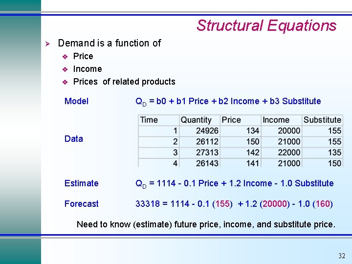
Structural Equations Ø Demand is a function of v v v Price Income Prices of related products Model QD = b 0 + b 1 Price + b 2 Income + b 3 Substitute Data Estimate QD = 1114 - 0. 1 Price + 1. 2 Income - 1. 0 Substitute Forecast 33318 = 1114 - 0. 1 (155) + 1. 2 (20000) - 1. 0 (160) Need to know (estimate) future price, income, and substitute price. 32

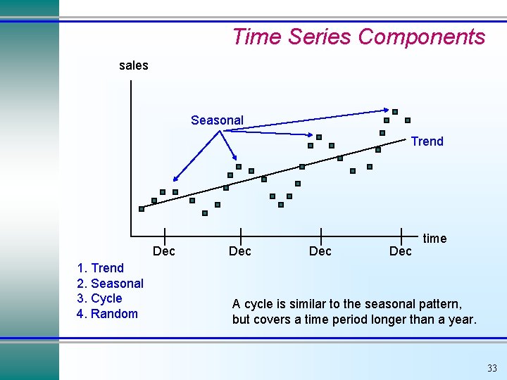
Time Series Components sales Seasonal Trend Dec 1. Trend 2. Seasonal 3. Cycle 4. Random Dec Dec time A cycle is similar to the seasonal pattern, but covers a time period longer than a year. 33

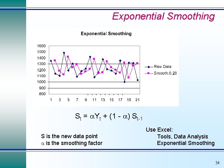
Exponential Smoothing St = Yt + (1 - ) St-1 S is the new data point is the smoothing factor Use Excel: Tools, Data Analysis Exponential Smoothing 34

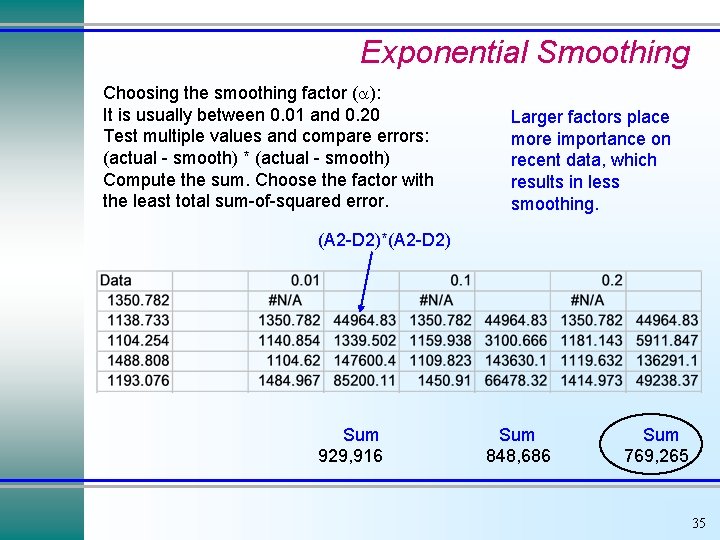
Exponential Smoothing Choosing the smoothing factor ( ): It is usually between 0. 01 and 0. 20 Test multiple values and compare errors: (actual - smooth) * (actual - smooth) Compute the sum. Choose the factor with the least total sum-of-squared error. Larger factors place more importance on recent data, which results in less smoothing. (A 2 -D 2)*(A 2 -D 2) Sum 929, 916 Sum 848, 686 Sum 769, 265 35

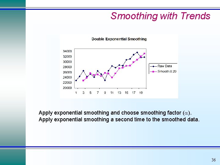
Smoothing with Trends Apply exponential smoothing and choose smoothing factor ( ). Apply exponential smoothing a second time to the smoothed data. 36

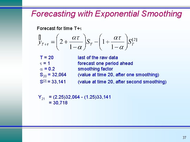
Forecasting with Exponential Smoothing Forecast for time T+ T = 20 =1 = 0. 2 S 20 = 32, 064 last of the raw data forecast one period ahead smoothing factor (value at time 20, after one smoothing) S[2] = 33, 141 (value at time 20, after second smoothing) Y 21 = (2. 25)32, 064 - (1. 25)33, 141 = 30, 718 37

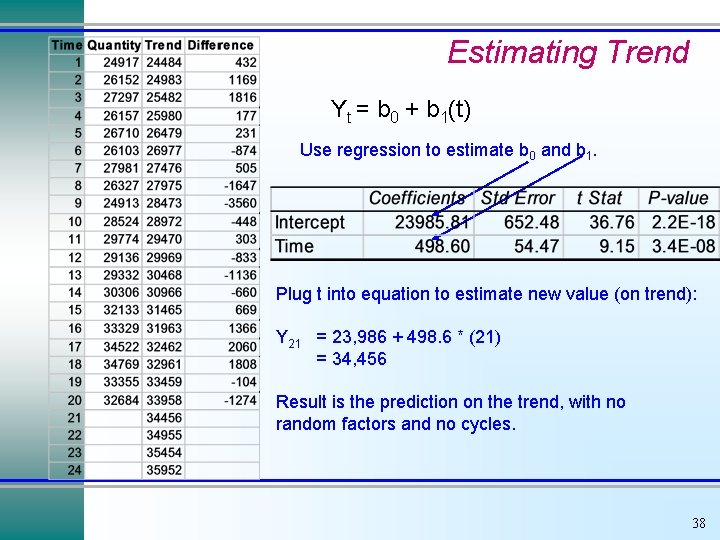
Estimating Trend Yt = b 0 + b 1(t) Use regression to estimate b 0 and b 1. Plug t into equation to estimate new value (on trend): Y 21 = 23, 986 + 498. 6 * (21) = 34, 456 Result is the prediction on the trend, with no random factors and no cycles. 38

An Overview of Decision Support Systems

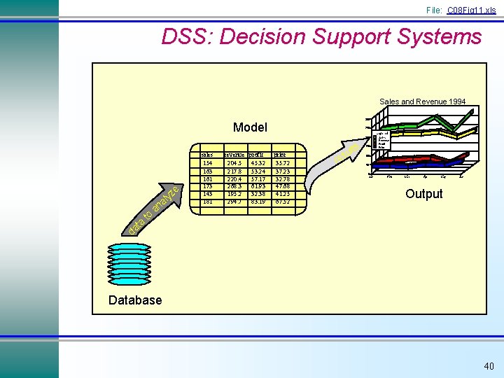
File: C 08 Fig 11. xls DSS: Decision Support Systems Sales and Revenue 1994 300 Model 250 Legend 200 ze y al a at to an sales 154 163 161 173 143 181 revenue profit 204. 5 45. 32 217. 8 53. 24 220. 4 57. 17 268. 3 61. 93 195. 2 32. 38 294. 7 83. 19 prior 35. 72 37. 23 32. 78 47. 68 41. 25 67. 52 lts r u es 150 Sales Revenue Profit Prior 100 50 0 Jan Feb Mar Apr May Jun Output d Database 40

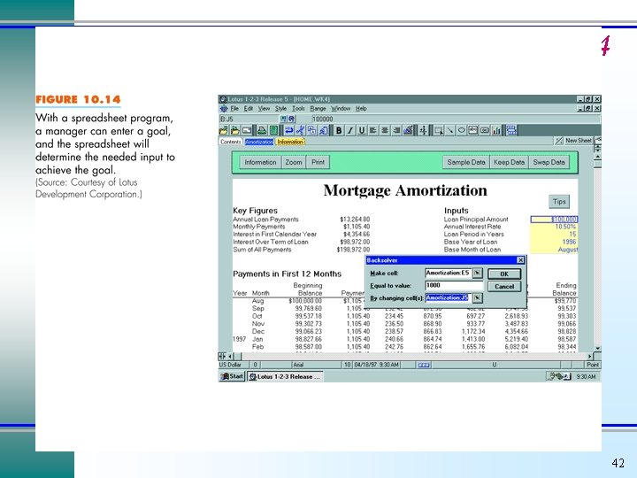
Characteristics of Decision Support Systems Ø Ø Ø Handle lots of data from various sources Report & presentation flexibility Text and graphics capabilities Support drill down analysis Complex analysis, statistics, and forecasting Optimization, satisficing, heuristics v v v Simulation What-if analysis Goal-seeking analysis 41

Figure 10. 14 42

Capabilities of a DSS Ø Ø Support all problem-solving phases Support different decision frequencies Support different problem structures Support various decision-making levels 43

The Model Base Ø Financial models v v Ø Statistical analysis models v v v Ø Ø Cash flow Internal rate of return Averages, standard deviations Correlations Regression analysis Graphical models Project management models 44

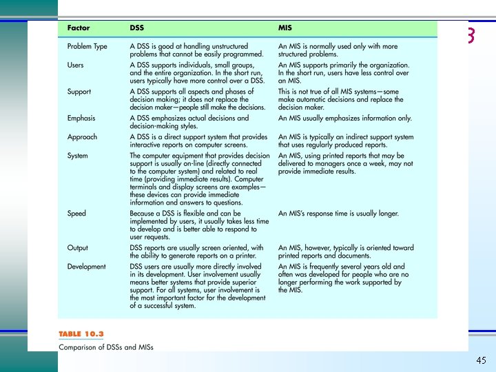
Table 10. 3 45

Group Decision Support Systems

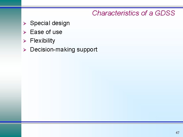
Characteristics of a GDSS Ø Ø Special design Ease of use Flexibility Decision-making support 47

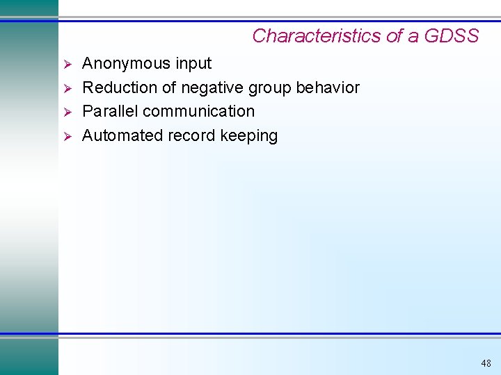
Characteristics of a GDSS Ø Ø Anonymous input Reduction of negative group behavior Parallel communication Automated record keeping 48

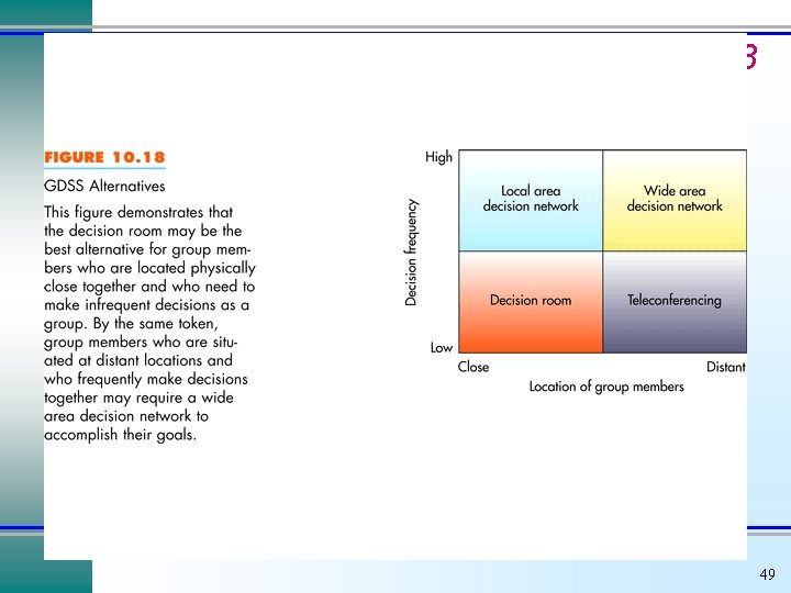
Figure 10. 18 49

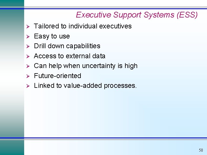
Executive Support Systems (ESS) Ø Ø Ø Ø Tailored to individual executives Easy to use Drill down capabilities Access to external data Can help when uncertainty is high Future-oriented Linked to value-added processes. 50

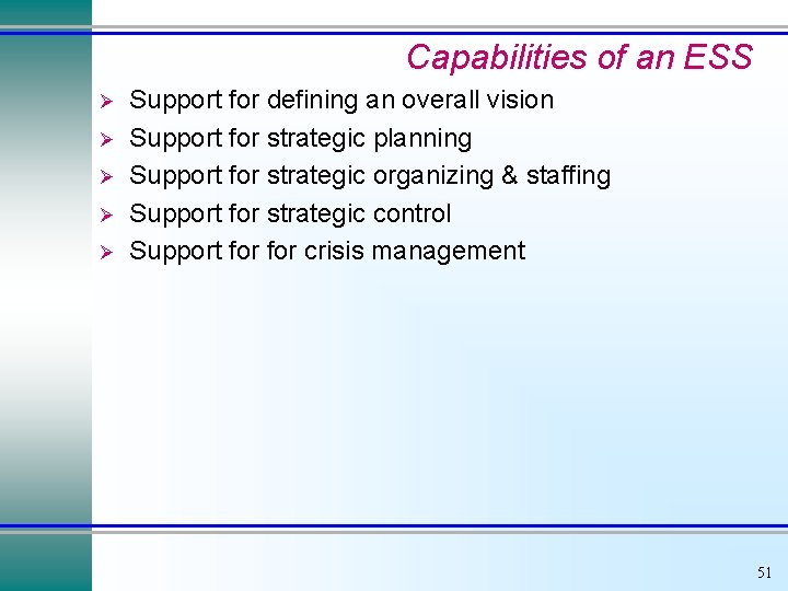
Capabilities of an ESS Ø Ø Ø Support for defining an overall vision Support for strategic planning Support for strategic organizing & staffing Support for strategic control Support for crisis management 51

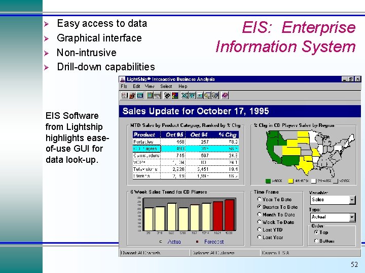
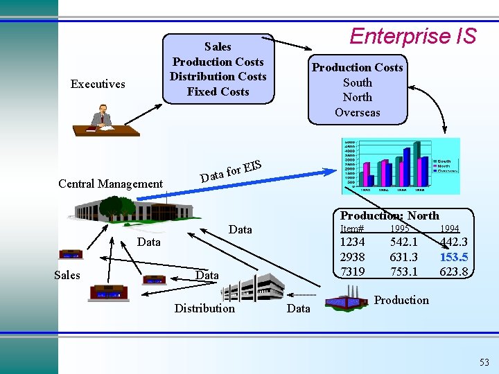
Ø Ø Easy access to data Graphical interface Non-intrusive Drill-down capabilities EIS: Enterprise Information System EIS Software from Lightship highlights easeof-use GUI for data look-up. 52

Enterprise IS Sales Production Costs Distribution Costs Fixed Costs Executives Central Management for Data Production Costs South North Overseas EIS Production: North Data Sales Data Distribution Data Item# 1995 1994 1234 2938 7319 542. 1 631. 3 753. 1 442. 3 153. 5 623. 8 Production 53