INF 5063 Programming heterogeneous multicore processors x 86

INF 5063: Programming heterogeneous multi-core processors x 86 and M-JPEG October 26, 2021

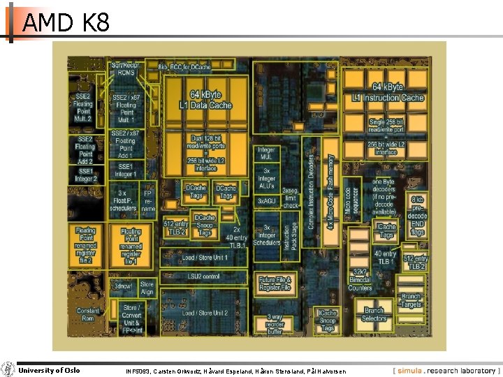
AMD K 8 University of Oslo INF 5063, Carsten Griwodz, Håvard Espeland, Håkon Stensland, Pål Halvorsen

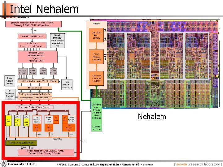
Intel Nehalem University of Oslo INF 5063, Carsten Griwodz, Håvard Espeland, Håkon Stensland, Pål Halvorsen

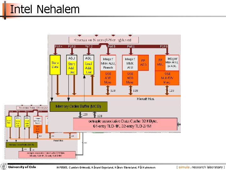
Intel Nehalem University of Oslo INF 5063, Carsten Griwodz, Håvard Espeland, Håkon Stensland, Pål Halvorsen

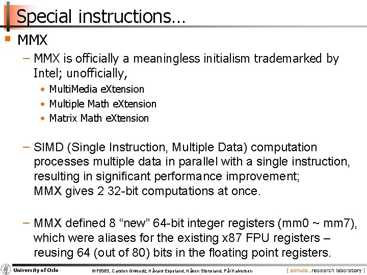
Special instructions… § MMX − MMX is officially a meaningless initialism trademarked by Intel; unofficially, • Multi. Media e. Xtension • Multiple Math e. Xtension • Matrix Math e. Xtension − SIMD (Single Instruction, Multiple Data) computation processes multiple data in parallel with a single instruction, resulting in significant performance improvement; MMX gives 2 32 -bit computations at once. − MMX defined 8 “new” 64 -bit integer registers (mm 0 ~ mm 7), which were aliases for the existing x 87 FPU registers – reusing 64 (out of 80) bits in the floating point registers. University of Oslo INF 5063, Carsten Griwodz, Håvard Espeland, Håkon Stensland, Pål Halvorsen

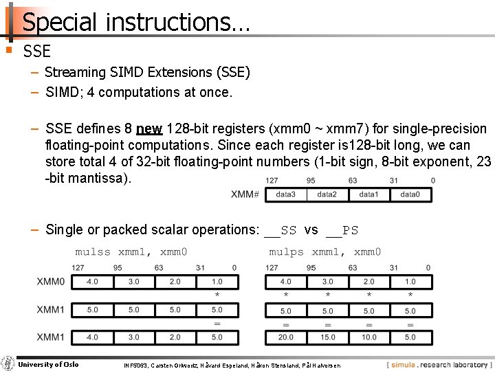
Special instructions… § SSE − Streaming SIMD Extensions (SSE) − SIMD; 4 computations at once. − SSE defines 8 new 128 -bit registers (xmm 0 ~ xmm 7) for single-precision floating-point computations. Since each register is 128 -bit long, we can store total 4 of 32 -bit floating-point numbers (1 -bit sign, 8 -bit exponent, 23 -bit mantissa). − Single or packed scalar operations: __SS vs __PS University of Oslo INF 5063, Carsten Griwodz, Håvard Espeland, Håkon Stensland, Pål Halvorsen

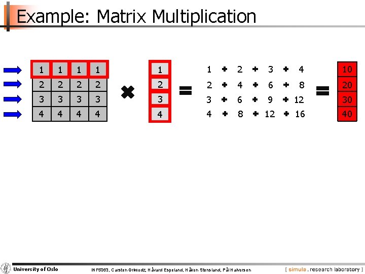
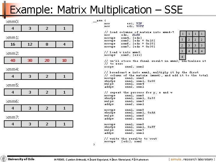
Example: Matrix Multiplication 1 1 1 2 3 4 10 2 2 2 4 6 8 20 3 3 3 6 9 12 30 4 4 4 8 12 16 40 University of Oslo INF 5063, Carsten Griwodz, Håvard Espeland, Håkon Stensland, Pål Halvorsen

Example: Matrix Multiplication - C #include <stdio. h> float elts[4][4] = {1, 1, 2, 2, 3, 3, 4, 4, 4, 4}; float vin[4] = {1, 2, 3, 4}; float vout[4]; void main(void) { vout[0] = elts[0][0] * vin[0] elts[0][2] * vin[2] + + elts[0][1] * vin[1] + elts[0][3] * vin[3]; vout[1] = elts[1][0] * vin[0] elts[1][2] * vin[2] + + elts[1][1] * vin[1] + elts[1][3] * vin[3]; vout[2] = elts[2][0] * vin[0] elts[2][2] * vin[2] + + elts[2][1] * vin[1] + elts[2][3] * vin[3]; vout[3] = elts[3][0] * vin[0] elts[3][2] * vin[2] + + elts[3][1] * vin[1] + elts[3][3] * vin[3]; printf("%f %fn", vout[0], vout[1], vout[2], vout[3]); } University of Oslo INF 5063, Carsten Griwodz, Håvard Espeland, Håkon Stensland, Pål Halvorsen

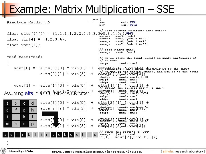
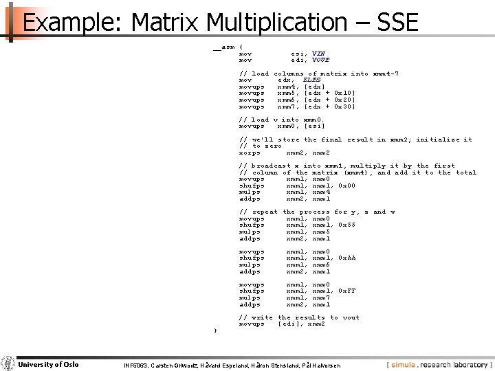
Example: Matrix Multiplication – SSE __asm { mov #include <stdio. h> esi, VIN edi, VOUT // load columns of matrix into xmm 4 -7 mov edx, ELTS float elts[4][4] = {1, 1, 2, 2, 3, 3, 4, 4, 4, 4}; movups xmm 4, [edx] movups xmm 5, [edx + float vin[4] = {1, 2, 3, 4}; movups xmm 6, [edx + movups xmm 7, [edx + float vout[4]; 0 x 10] 0 x 20] 0 x 30] // load v into xmm 0. movups xmm 0, [esi] void main(void) { vout[0] = elts[0][0] * vin[0] elts[0][2] * vin[2] vout[1] = // we'll store the final result in xmm 2; initialize it // to zero xorps xmm 2, xmm 2 elts[1][0] * vin[0] elts[1][2] * vin[2] + + elts[0][1] vin[1] // broadcast x*into xmm 1, + multiply it by the first // column of the matrix (xmm 4), and add it to the total movups xmm 1, xmm 0 elts[0][3] * vin[3]; + + elts[1][1] * vin[1] + // repeat the process for y, movups xmm 1, xmm 0 elts[1][3] * vin[3]; shufps xmm 1, 0 x 55 Assuming elts in a COLUMN-MAJOR order: vout[2] b c d= a e f i h j k l vout[3] = n o p m a g e i n b f elts[2][0] * vin[0] elts[2][2] * vin[2] + + elts[3][0] * vin[0] elts[3][2] * vin[2] j n c g k o d h + + l shufps mulps addps xmm 1, 0 x 00 xmm 1, xmm 4 xmm 2, xmm 1 mulps addps xmm 1, xmm 5 xmm 2, xmm 1 addps xmm 2, xmm 1 movups xmm 1, xmm 0 z and w elts[2][1] * vin[1] + movups xmm 1, xmm 0 shufps xmm 1, 0 x. AA elts[2][3] * vin[3]; mulps xmm 1, xmm 6 elts[3][1] * vin[1] + shufps xmm 1, 0 x. FF mulps xmm 1, xmm 7 elts[3][3] * vin[3]; addps xmm 2, xmm 1 // write the results to vout [edi], xmm 2 p movups } vout[1], vout[2], vout[3]); printf("%f %fn", vout[0], } University of Oslo INF 5063, Carsten Griwodz, Håvard Espeland, Håkon Stensland, Pål Halvorsen

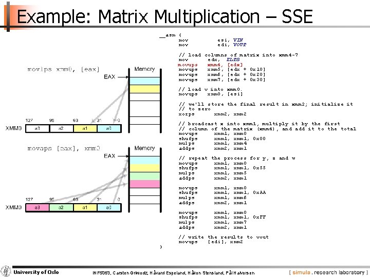
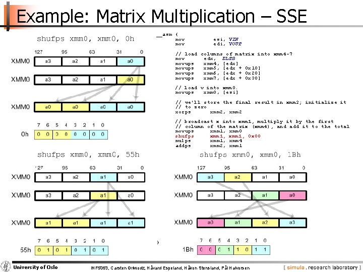
Example: Matrix Multiplication – SSE __asm { mov esi, VIN edi, VOUT // load columns of matrix into xmm 4 -7 mov edx, ELTS movups xmm 4, [edx] movups xmm 5, [edx + 0 x 10] movups xmm 6, [edx + 0 x 20] movups xmm 7, [edx + 0 x 30] // load v into xmm 0. movups xmm 0, [esi] // we'll store the final result in xmm 2; initialize it // to zero xorps xmm 2, xmm 2 // broadcast x into xmm 1, multiply it by the first // column of the matrix (xmm 4), and add it to the total movups xmm 1, xmm 0 shufps xmm 1, 0 x 00 mulps xmm 1, xmm 4 addps xmm 2, xmm 1 // repeat the process for y, z and w movups xmm 1, xmm 0 shufps xmm 1, 0 x 55 mulps xmm 1, xmm 5 addps xmm 2, xmm 1 } University of Oslo movups shufps mulps addps xmm 1, xmm 2, xmm 0 xmm 1, 0 x. AA xmm 6 xmm 1 movups shufps mulps addps xmm 1, xmm 2, xmm 0 xmm 1, 0 x. FF xmm 7 xmm 1 // write the results to vout movups [edi], xmm 2 INF 5063, Carsten Griwodz, Håvard Espeland, Håkon Stensland, Pål Halvorsen

Example: Matrix Multiplication – SSE __asm { mov esi, VIN edi, VOUT // load columns of matrix into xmm 4 -7 mov edx, ELTS movups xmm 4, [edx] movups xmm 5, [edx + 0 x 10] movups xmm 6, [edx + 0 x 20] movups xmm 7, [edx + 0 x 30] // load v into xmm 0. movups xmm 0, [esi] // we'll store the final result in xmm 2; initialize it // to zero xorps xmm 2, xmm 2 // broadcast x into xmm 1, multiply it by the first // column of the matrix (xmm 4), and add it to the total movups xmm 1, xmm 0 shufps xmm 1, 0 x 00 mulps xmm 1, xmm 4 addps xmm 2, xmm 1 // repeat the process for y, z and w movups xmm 1, xmm 0 shufps xmm 1, 0 x 55 mulps xmm 1, xmm 5 addps xmm 2, xmm 1 } University of Oslo movups shufps mulps addps xmm 1, xmm 2, xmm 0 xmm 1, 0 x. AA xmm 6 xmm 1 movups shufps mulps addps xmm 1, xmm 2, xmm 0 xmm 1, 0 x. FF xmm 7 xmm 1 // write the results to vout movups [edi], xmm 2 INF 5063, Carsten Griwodz, Håvard Espeland, Håkon Stensland, Pål Halvorsen

Example: Matrix Multiplication – SSE __asm { mov esi, VIN edi, VOUT // load columns of matrix into xmm 4 -7 mov edx, ELTS movups xmm 4, [edx] movups xmm 5, [edx + 0 x 10] movups xmm 6, [edx + 0 x 20] movups xmm 7, [edx + 0 x 30] // load v into xmm 0. movups xmm 0, [esi] // we'll store the final result in xmm 2; initialize it // to zero xorps xmm 2, xmm 2 // broadcast x into xmm 1, multiply it by the first // column of the matrix (xmm 4), and add it to the total movups xmm 1, xmm 0 shufps xmm 1, 0 x 00 mulps xmm 1, xmm 4 addps xmm 2, xmm 1 // repeat the process for y, z and w movups xmm 1, xmm 0 shufps xmm 1, 0 x 55 mulps xmm 1, xmm 5 addps xmm 2, xmm 1 } University of Oslo movups shufps mulps addps xmm 1, xmm 2, xmm 0 xmm 1, 0 x. AA xmm 6 xmm 1 movups shufps mulps addps xmm 1, xmm 2, xmm 0 xmm 1, 0 x. FF xmm 7 xmm 1 // write the results to vout movups [edi], xmm 2 INF 5063, Carsten Griwodz, Håvard Espeland, Håkon Stensland, Pål Halvorsen

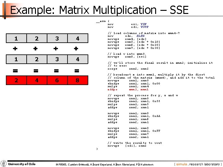
Example: Matrix Multiplication – SSE __asm { mov 1 1 1 2 2 4 3 3 9 esi, VIN edi, VOUT // load columns of matrix into xmm 4 -7 mov edx, ELTS movups xmm 4, [edx] movups xmm 5, [edx + 0 x 10] movups xmm 6, [edx + 0 x 20] movups xmm 7, [edx + 0 x 30] 4 // load v into xmm 0. movups xmm 0, [esi] 4 // we'll store the final result in xmm 2; initialize it // to zero xorps xmm 2, xmm 2 // broadcast x into xmm 1, multiply it by the first // column of the matrix (xmm 4), and add it to the total movups xmm 1, xmm 0 shufps xmm 1, 0 x 00 mulps xmm 1, xmm 4 addps xmm 2, xmm 1 16 // repeat the process for y, z and w movups xmm 1, xmm 0 shufps xmm 1, 0 x 55 mulps xmm 1, xmm 5 addps xmm 2, xmm 1 } University of Oslo movups shufps mulps addps xmm 1, xmm 2, xmm 0 xmm 1, 0 x. AA xmm 6 xmm 1 movups shufps mulps addps xmm 1, xmm 2, xmm 0 xmm 1, 0 x. FF xmm 7 xmm 1 // write the results to vout movups [edi], xmm 2 INF 5063, Carsten Griwodz, Håvard Espeland, Håkon Stensland, Pål Halvorsen

Example: Matrix Multiplication – SSE __asm { mov 1 1 2 2 2 4 3 3 6 esi, VIN edi, VOUT // load columns of matrix into xmm 4 -7 mov edx, ELTS movups xmm 4, [edx] movups xmm 5, [edx + 0 x 10] movups xmm 6, [edx + 0 x 20] movups xmm 7, [edx + 0 x 30] 4 // load v into xmm 0. movups xmm 0, [esi] 4 // we'll store the final result in xmm 2; initialize it // to zero xorps xmm 2, xmm 2 // broadcast x into xmm 1, multiply it by the first // column of the matrix (xmm 4), and add it to the total movups xmm 1, xmm 0 shufps xmm 1, 0 x 00 mulps xmm 1, xmm 4 addps xmm 2, xmm 1 8 // repeat the process for y, z and w movups xmm 1, xmm 0 shufps xmm 1, 0 x 55 mulps xmm 1, xmm 5 addps xmm 2, xmm 1 } University of Oslo movups shufps mulps addps xmm 1, xmm 2, xmm 0 xmm 1, 0 x. AA xmm 6 xmm 1 movups shufps mulps addps xmm 1, xmm 2, xmm 0 xmm 1, 0 x. FF xmm 7 xmm 1 // write the results to vout movups [edi], xmm 2 INF 5063, Carsten Griwodz, Håvard Espeland, Håkon Stensland, Pål Halvorsen

Example: Matrix Multiplication – SSE xmm 0: 4 3 2 1 __asm { mov // load columns of matrix into xmm 4 -7 mov edx, ELTS movups xmm 4, [edx] movups xmm 5, [edx + 0 x 10] movups xmm 6, [edx + 0 x 20] movups xmm 7, [edx + 0 x 30] xmm 1: 12 16 1 2 8 3 4 12 1 2 6 9 3 4 1 3 6 2 4 8 2 3 1 4 // load v into xmm 0. movups xmm 0, [esi] xmm 2: 12 24 40 0 4 18 30 0 3 9 12 20 0 2 6 3 2 1 // repeat the process for y, z and w movups xmm 1, xmm 0 shufps xmm 1, 0 x 55 mulps xmm 1, xmm 5 addps xmm 2, xmm 1 xmm 6: 4 xmm 7: 4 } University of Oslo 1 12 2 23 3 34 4 // broadcast x into xmm 1, multiply it by the first // column of the matrix (xmm 4), and add it to the total movups xmm 1, xmm 0 shufps xmm 1, 0 x 00 mulps xmm 1, xmm 4 addps xmm 2, xmm 1 xmm 5: 4 1 4 // we'll store the final result in xmm 2; initialize it // to zero xorps xmm 2, xmm 2 10 0 1 3 6 xmm 4: 4 esi, VIN edi, VOUT movups shufps mulps addps xmm 1, xmm 2, xmm 0 xmm 1, 0 x. AA xmm 6 xmm 1 movups shufps mulps addps xmm 1, xmm 2, xmm 0 xmm 1, 0 x. FF xmm 7 xmm 1 // write the results to vout movups [edi], xmm 2 INF 5063, Carsten Griwodz, Håvard Espeland, Håkon Stensland, Pål Halvorsen

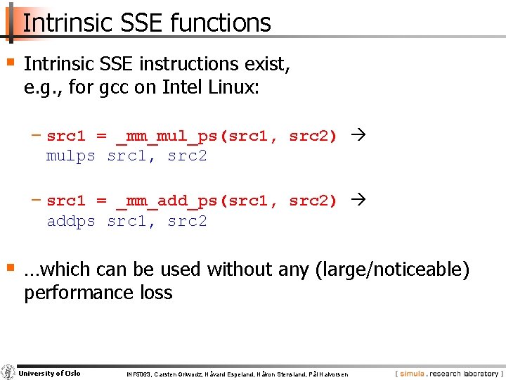
Intrinsic SSE functions § Intrinsic SSE instructions exist, e. g. , for gcc on Intel Linux: − src 1 = _mm_mul_ps(src 1, src 2) mulps src 1, src 2 − src 1 = _mm_add_ps(src 1, src 2) addps src 1, src 2 § …which can be used without any (large/noticeable) performance loss University of Oslo INF 5063, Carsten Griwodz, Håvard Espeland, Håkon Stensland, Pål Halvorsen

(M-) JPEG The very short, turbo fast introduction

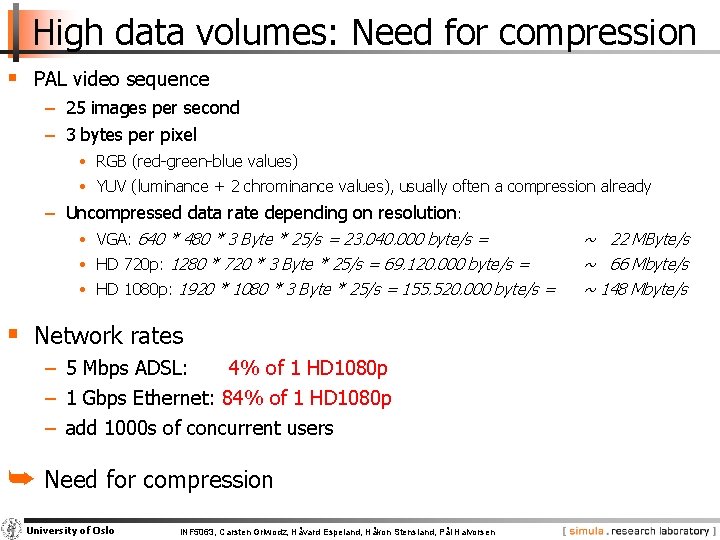
High data volumes: Need for compression § PAL video sequence − 25 images per second − 3 bytes per pixel • RGB (red-green-blue values) • YUV (luminance + 2 chrominance values), usually often a compression already − Uncompressed data rate depending on resolution: • VGA: 640 * 480 * 3 Byte * 25/s = 23. 040. 000 byte/s = • HD 720 p: 1280 * 720 * 3 Byte * 25/s = 69. 120. 000 byte/s = • HD 1080 p: 1920 * 1080 * 3 Byte * 25/s = 155. 520. 000 byte/s = § Network rates − 5 Mbps ADSL: 4% of 1 HD 1080 p − 1 Gbps Ethernet: 84% of 1 HD 1080 p − add 1000 s of concurrent users ➥ Need for compression University of Oslo INF 5063, Carsten Griwodz, Håvard Espeland, Håkon Stensland, Pål Halvorsen ~ 22 MByte/s ~ 66 Mbyte/s ~ 148 Mbyte/s

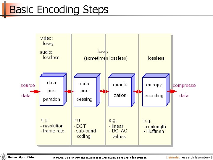
Basic Encoding Steps University of Oslo INF 5063, Carsten Griwodz, Håvard Espeland, Håkon Stensland, Pål Halvorsen

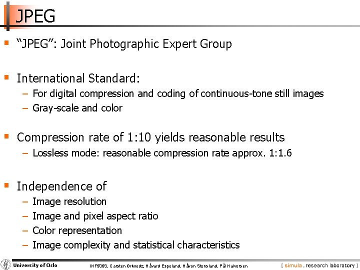
JPEG § “JPEG”: Joint Photographic Expert Group § International Standard: − For digital compression and coding of continuous-tone still images − Gray-scale and color § Compression rate of 1: 10 yields reasonable results − Lossless mode: reasonable compression rate approx. 1: 1. 6 § Independence of − − Image resolution Image and pixel aspect ratio Color representation Image complexity and statistical characteristics University of Oslo INF 5063, Carsten Griwodz, Håvard Espeland, Håkon Stensland, Pål Halvorsen

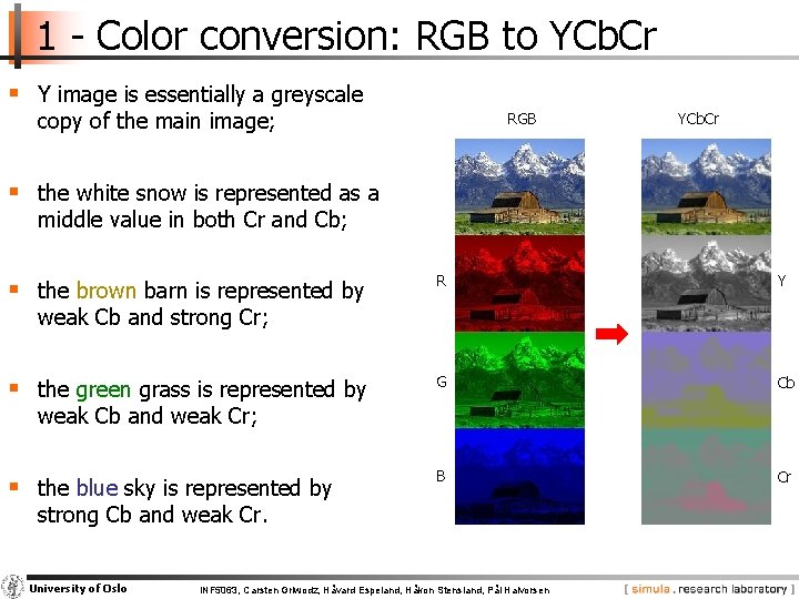
1 - Color conversion: RGB to YCb. Cr § Y image is essentially a greyscale copy of the main image; RGB YCb. Cr § the white snow is represented as a middle value in both Cr and Cb; § the brown barn is represented by R Y § the green grass is represented by G Cb § the blue sky is represented by B Cr weak Cb and strong Cr; weak Cb and weak Cr; strong Cb and weak Cr. University of Oslo INF 5063, Carsten Griwodz, Håvard Espeland, Håkon Stensland, Pål Halvorsen

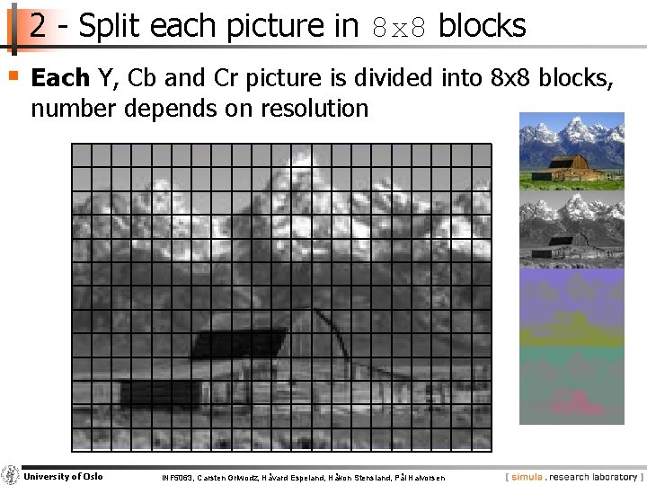
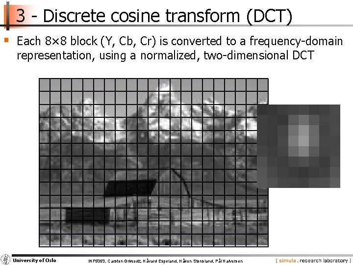
2 - Split each picture in 8 x 8 blocks § Each Y, Cb and Cr picture is divided into 8 x 8 blocks, number depends on resolution University of Oslo INF 5063, Carsten Griwodz, Håvard Espeland, Håkon Stensland, Pål Halvorsen

3 - Discrete cosine transform (DCT) § Each 8× 8 block (Y, Cb, Cr) is converted to a frequency-domain representation, using a normalized, two-dimensional DCT University of Oslo INF 5063, Carsten Griwodz, Håvard Espeland, Håkon Stensland, Pål Halvorsen

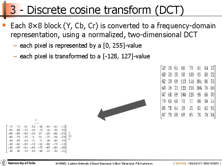
3 - Discrete cosine transform (DCT) § Each 8× 8 block (Y, Cb, Cr) is converted to a frequency-domain representation, using a normalized, two-dimensional DCT − each pixel is represented by a [0, 255]-value − each pixel is transformed to a [-128, 127]-value University of Oslo INF 5063, Carsten Griwodz, Håvard Espeland, Håkon Stensland, Pål Halvorsen

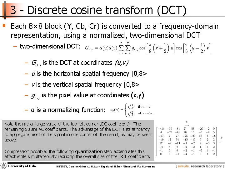
3 - Discrete cosine transform (DCT) § Each 8× 8 block (Y, Cb, Cr) is converted to a frequency-domain representation, using a normalized, two-dimensional DCT − two-dimensional DCT: − Gu, v is the DCT at coordinates (u, v) − u is the horizontal spatial frequency [0, 8> − v is the vertical spatial frequency [0, 8> − gx, y is the pixel value at coordinates (x, y) − α is a normalizing function: Note the rather large value of the top-left corner (DC coefficient). The remaining 63 are AC coefficients. The advantage of the DCT is its tendency to aggregate most of the signal in one corner of the result, as may be seen above. Compression possible: the following quantization step accentuates this effect while simultaneously reducing the overall size of the DCT coefficients University of Oslo INF 5063, Carsten Griwodz, Håvard Espeland, Håkon Stensland, Pål Halvorsen

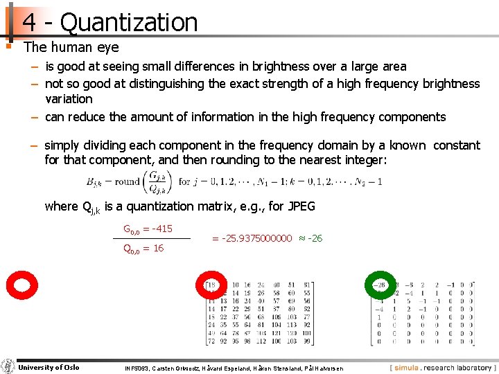
4 - Quantization § The human eye − is good at seeing small differences in brightness over a large area − not so good at distinguishing the exact strength of a high frequency brightness variation − can reduce the amount of information in the high frequency components − simply dividing each component in the frequency domain by a known constant for that component, and then rounding to the nearest integer: where Qj, k is a quantization matrix, e. g. , for JPEG G 0, 0 = -415 Q 0, 0 = 16 University of Oslo = -25. 9375000000 ≈ -26 INF 5063, Carsten Griwodz, Håvard Espeland, Håkon Stensland, Pål Halvorsen

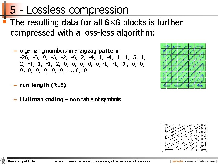
5 - Lossless compression § The resulting data for all 8× 8 blocks is further compressed with a loss-less algorithm: − organizing numbers in a zigzag pattern: -26, -3, 0, -3, -2, -6, 2, -4, 1, 1, 5, 1, 2, -1, 1, -1, 2, 0, 0, 0, -1, 0 , 0, 0, …. , 0, 0 − run-length (RLE) − Huffman coding – own table of symbols University of Oslo INF 5063, Carsten Griwodz, Håvard Espeland, Håkon Stensland, Pål Halvorsen

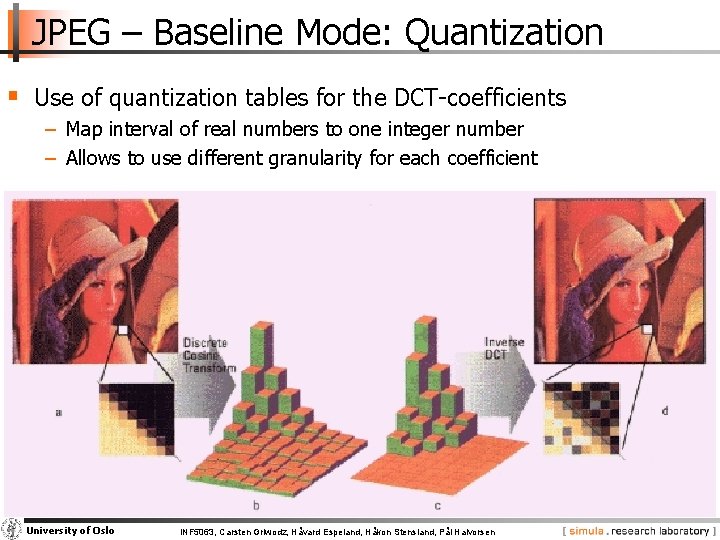
JPEG – Baseline Mode: Quantization § Use of quantization tables for the DCT-coefficients − Map interval of real numbers to one integer number − Allows to use different granularity for each coefficient University of Oslo INF 5063, Carsten Griwodz, Håvard Espeland, Håkon Stensland, Pål Halvorsen

Motion JPEG § Use series of JPEG frames to encode video § Pro − − − − Lossless mode Frame-accurate seeking Arbitrary frame rates Arbitrary frame skipping Scaling through progressive mode Min transmission delay = 1/framerate Supported by popular frame grabbers – – – editing advantage playback advantage distribution advantage conferencing advantage § Contra − Series of JPEG-compressed images − No standard, no specification • Worse, several competing quasi-standards − No relation to audio − No inter-frame compression University of Oslo INF 5063, Carsten Griwodz, Håvard Espeland, Håkon Stensland, Pål Halvorsen