Identifying Ancestry Informative Markers via the Singular Value

Identifying Ancestry Informative Markers via the Singular Value Decomposition Petros Drineas Rensselaer Polytechnic Institute Computer Science Department To access my web page: drineas

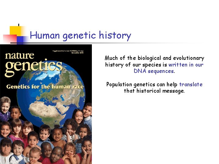
Human genetic history Much of the biological and evolutionary history of our species is written in our DNA sequences. Population genetics can help translate that historical message.

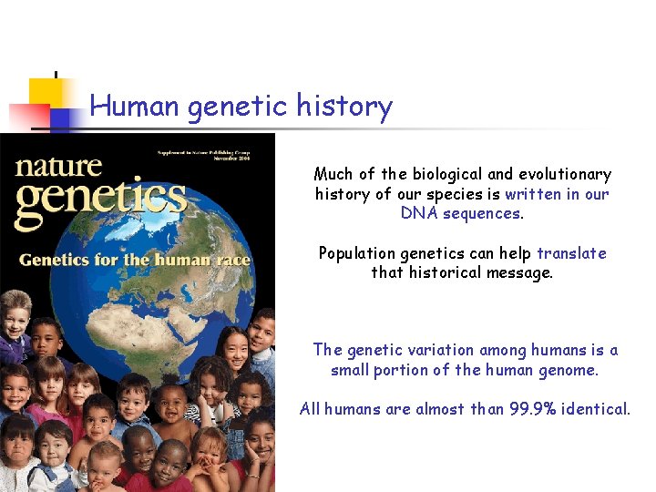
Human genetic history Much of the biological and evolutionary history of our species is written in our DNA sequences. Population genetics can help translate that historical message. The genetic variation among humans is a small portion of the human genome. All humans are almost than 99. 9% identical.

Our objective Develop unsupervised, efficient algorithms for the selection of a small set of genetic markers that can be used to Ø capture population structure, and Ø predict individual ancestry.

Our objective Develop unsupervised, efficient algorithms for the selection of a small set of genetic markers that can be used to Ø capture population structure, and Ø predict individual ancestry. To this end, we employ matrix algorithms and matrix decompositions such as Ø the Singular Value Decomposition (SVD), and Ø the CX decomposition. We provide the first unsupervised algorithm for selecting of such markers.

Overview • Basic genetics background • The Singular Value Decomposition (SVD) • The CX decomposition • Selecting Ancestry Informative Markers Ø The Hap. Map data Ø A worldwide set of populations Ø An admixed population

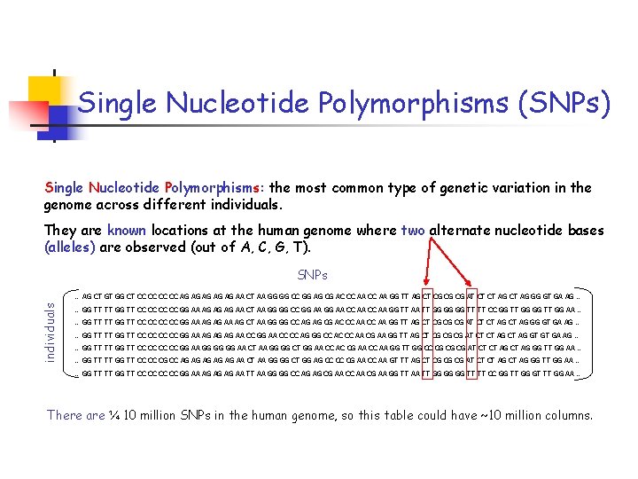
Single Nucleotide Polymorphisms (SNPs) Single Nucleotide Polymorphisms: the most common type of genetic variation in the genome across different individuals. They are known locations at the human genome where two alternate nucleotide bases (alleles) are observed (out of A, C, G, T). SNPs individuals … AG CT GT GG CT CC CC AG AG AG AA CT AA GG GG CC GG AG CG AC CC AA GG TT AG CT CG CG CG AT CT CT AG GG GT GA AG … … GG TT TT GG TT CC CC GG AA AG AG AG AA CT AA GG GG CC GG AA CC AA GG TT AA TT GG GG GG TT TT CC GG TT GG AA … … GG TT TT GG TT CC CC GG AA AG AG AA AG CT AA GG GG CC AG AG CG AC CC AA GG TT AG CT CG CG CG AT CT CT AG GG GT GA AG … … GG TT TT GG TT CC CC GG AA AG AG AG AA CC GG AA CC CC AG GG CC AC CC AA CG AA GG TT AG CT CG CG CG AT CT CT AG GT GT GA AG … … GG TT TT GG TT CC CC GG AA GG GG GG AA CT AA GG GG CT GG AA CC AC CG AA CC AA GG TT GG CC CG CG CG AT CT CT AG GG TT GG AA … … GG TT TT GG TT CC CC CG CC AG AG AG AA CT AA GG GG CT GG AG CC CC CG AA CC AA GT TT AG CT CG CG CG AT CT CT AG GG TT GG AA … … GG TT TT GG TT CC CC GG AA AG AG AG AA TT AA GG GG CC AG AG CG AA CC AA CG AA GG TT AA TT GG GG GG TT TT CC GG TT GG GT TT GG AA … There are ¼ 10 million SNPs in the human genome, so this table could have ~10 million columns.

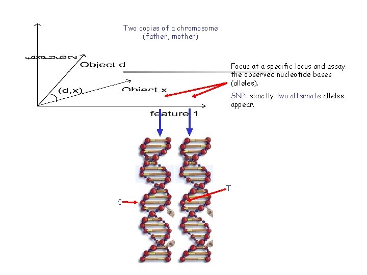
Two copies of a chromosome (father, mother) Focus at a specific locus and assay the observed nucleotide bases (alleles). SNP: exactly two alternate alleles appear. T C

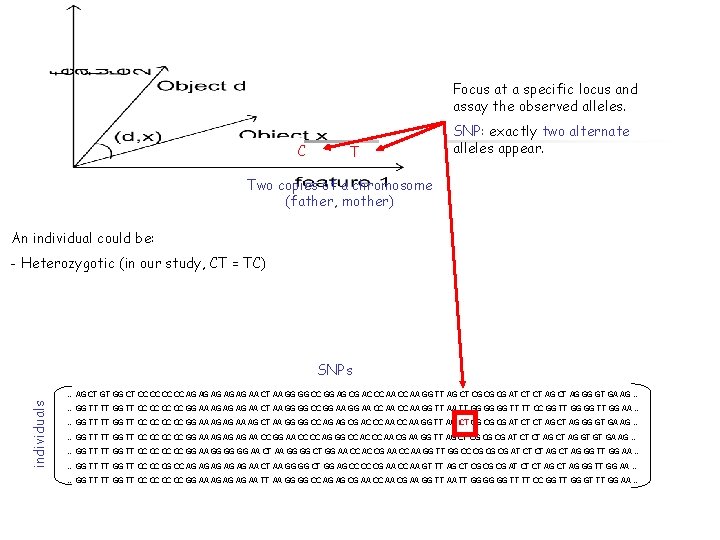
Focus at a specific locus and assay the observed alleles. C T SNP: exactly two alternate alleles appear. Two copies of a chromosome (father, mother) An individual could be: - Heterozygotic (in our study, CT = TC) SNPs individuals … AG CT GT GG CT CC CC AG AG AG AA CT AA GG GG CC GG AG CG AC CC AA GG TT AG CT CG CG CG AT CT CT AG GG GT GA AG … … GG TT TT GG TT CC CC GG AA AG AG AG AA CT AA GG GG CC GG AA CC AA GG TT AA TT GG GG GG TT TT CC GG TT GG AA … … GG TT TT GG TT CC CC GG AA AG AG AA AG CT AA GG GG CC AG AG CG AC CC AA GG TT AG CT CG CG CG AT CT CT AG GG GT GA AG … … GG TT TT GG TT CC CC GG AA AG AG AG AA CC GG AA CC CC AG GG CC AC CC AA CG AA GG TT AG CT CG CG CG AT CT CT AG GT GT GA AG … … GG TT TT GG TT CC CC GG AA GG GG GG AA CT AA GG GG CT GG AA CC AC CG AA CC AA GG TT GG CC CG CG CG AT CT CT AG GG TT GG AA … … GG TT TT GG TT CC CC CG CC AG AG AG AA CT AA GG GG CT GG AG CC CC CG AA CC AA GT TT AG CT CG CG CG AT CT CT AG GG TT GG AA … … GG TT TT GG TT CC CC GG AA AG AG AG AA TT AA GG GG CC AG AG CG AA CC AA CG AA GG TT AA TT GG GG GG TT TT CC GG TT GG GT TT GG AA …

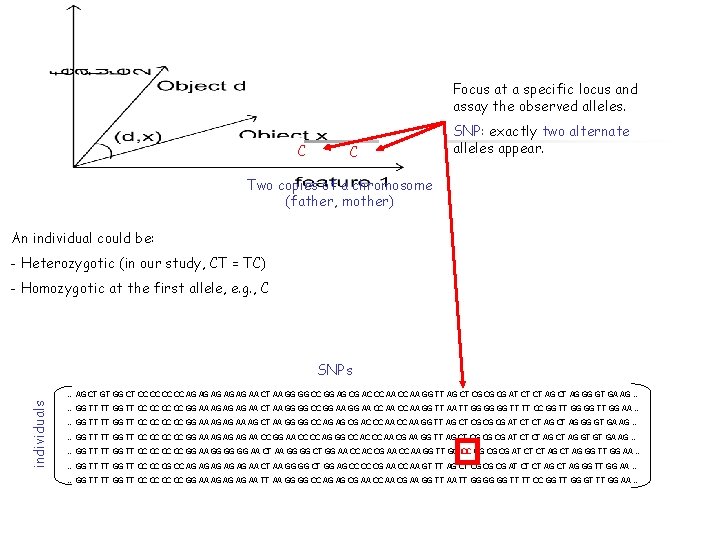
Focus at a specific locus and assay the observed alleles. C C SNP: exactly two alternate alleles appear. Two copies of a chromosome (father, mother) An individual could be: - Heterozygotic (in our study, CT = TC) - Homozygotic at the first allele, e. g. , C SNPs individuals … AG CT GT GG CT CC CC AG AG AG AA CT AA GG GG CC GG AG CG AC CC AA GG TT AG CT CG CG CG AT CT CT AG GG GT GA AG … … GG TT TT GG TT CC CC GG AA AG AG AG AA CT AA GG GG CC GG AA CC AA GG TT AA TT GG GG GG TT TT CC GG TT GG AA … … GG TT TT GG TT CC CC GG AA AG AG AA AG CT AA GG GG CC AG AG CG AC CC AA GG TT AG CT CG CG CG AT CT CT AG GG GT GA AG … … GG TT TT GG TT CC CC GG AA AG AG AG AA CC GG AA CC CC AG GG CC AC CC AA CG AA GG TT AG CT CG CG CG AT CT CT AG GT GT GA AG … … GG TT TT GG TT CC CC GG AA GG GG GG AA CT AA GG GG CT GG AA CC AC CG AA CC AA GG TT GG CC CG CG CG AT CT CT AG GG TT GG AA … … GG TT TT GG TT CC CC CG CC AG AG AG AA CT AA GG GG CT GG AG CC CC CG AA CC AA GT TT AG CT CG CG CG AT CT CT AG GG TT GG AA … … GG TT TT GG TT CC CC GG AA AG AG AG AA TT AA GG GG CC AG AG CG AA CC AA CG AA GG TT AA TT GG GG GG TT TT CC GG TT GG GT TT GG AA …

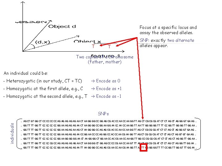
Focus at a specific locus and assay the observed alleles. T T SNP: exactly two alternate alleles appear. Two copies of a chromosome (father, mother) An individual could be: - Heterozygotic (in our study, CT = TC) à Encode as 0 - Homozygotic at the first allele, e. g. , C à Encode as +1 - Homozygotic at the second allele, e. g. , T à Encode as -1 SNPs individuals … AG CT GT GG CT CC CC AG AG AG AA CT AA GG GG CC GG AG CG AC CC AA GG TT AG CT CG CG CG AT CT CT AG GG GT GA AG … … GG TT TT GG TT CC CC GG AA AG AG AG AA CT AA GG GG CC GG AA CC AA GG TT AA TT GG GG GG TT TT CC GG TT GG AA … … GG TT TT GG TT CC CC GG AA AG AG AA AG CT AA GG GG CC AG AG CG AC CC AA GG TT AG CT CG CG CG AT CT CT AG GG GT GA AG … … GG TT TT GG TT CC CC GG AA AG AG AG AA CC GG AA CC CC AG GG CC AC CC AA CG AA GG TT AG CT CG CG CG AT CT CT AG GT GT GA AG … … GG TT TT GG TT CC CC GG AA GG GG GG AA CT AA GG GG CT GG AA CC AC CG AA CC AA GG TT GG CC CG CG CG AT CT CT AG GG TT GG AA … … GG TT TT GG TT CC CC CG CC AG AG AG AA CT AA GG GG CT GG AG CC CC CG AA CC AA GT TT AG CT CG CG CG AT CT CT AG GG TT GG AA … … GG TT TT GG TT CC CC GG AA AG AG AG AA TT AA GG GG CC AG AG CG AA CC AA CG AA GG TT AA TT GG GG GG TT TT CC GG TT GG GT TT GG AA …

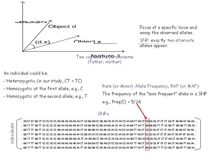
Focus at a specific locus and assay the observed alleles. SNP: exactly two alternate alleles appear. Two copies of a chromosome (father, mother) An individual could be: - Heterozygotic (in our study, CT = TC) - Homozygotic at the first allele, e. g. , C - Homozygotic at the second allele, e. g. , T Rare (or Minor) Allele Frequency, RAF (or MAF): The frequency of the “less frequent” allele in a SNP e. g. , freq(C) = 5/14. SNPs individuals … AG CT GT GG CT CC CC AG AG AG AA CT AA GG GG CC GG AG CG AC CC AA GG TT AG CT CG CG CG AT CT CT AG GG GT GA AG … … GG TT TT GG TT CC CC GG AA AG AG AG AA CT AA GG GG CC GG AA CC AA GG TT AA TT GG GG GG TT TT CC GG TT GG AA … … GG TT TT GG TT CC CC GG AA AG AG AA AG CT AA GG GG CC AG AG CG AC CC AA GG TT AG CT CG CG CG AT CT CT AG GG GT GA AG … … GG TT TT GG TT CC CC GG AA AG AG AG AA CC GG AA CC CC AG GG CC AC CC AA CG AA GG TT AG CT CG CG CG AT CT CT AG GT GT GA AG … … GG TT TT GG TT CC CC GG AA GG GG GG AA CT AA GG GG CT GG AA CC AC CG AA CC AA GG TT GG CC CG CG CG AT CT CT AG GG TT GG AA … … GG TT TT GG TT CC CC CG CC AG AG AG AA CT AA GG GG CT GG AG CC CC CG AA CC AA GT TT AG CT CG CG CG AT CT CT AG GG TT GG AA … … GG TT TT GG TT CC CC GG AA AG AG AG AA TT AA GG GG CC AG AG CG AA CC AA CG AA GG TT AA TT GG GG GG TT TT CC GG TT GG GT TT GG AA …

Population Genetics 101 Genetic diversity and population (sub)structure is caused by… • Mutations are changes to the base pair sequence of the DNA. • Natural selection Genotypes that correspond to favorable traits and are heritable become more common in successive generations of a population of reproducing organisms.

Population Genetics 101 Genetic diversity and population (sub)structure is caused by… • Mutations are changes to the base pair sequence of the DNA. • Natural selection Genotypes that correspond to favorable traits and are heritable become more common in successive generations of a population of reproducing organisms. Mutations increase genetic diversity. Under natural selection, beneficial mutations increase in frequency, and vice versa.

Population Genetics 101 (cont’d) • Genetic drift Sampling effects on evolution! Example: say that the RAF of a SNP in a small population is p. The offspring generation would (in expectation) have a RAF of p as well for the same SNP. In reality, it will have a RAF of p’ (a drifted frequency) … • Gene flow Transfer of alleles between populations.

Population Genetics 101 (cont’d) • Genetic drift Sampling effects on evolution! Example: say that the RAF of a SNP in a small population is p. The offspring generation would (in expectation) have a RAF of p as well for the same SNP. In reality, it will have a RAF of p’ (a drifted frequency) … • Gene flow Transfer of alleles between populations. Genetic drift are a stronger force than natural selection in small populations.

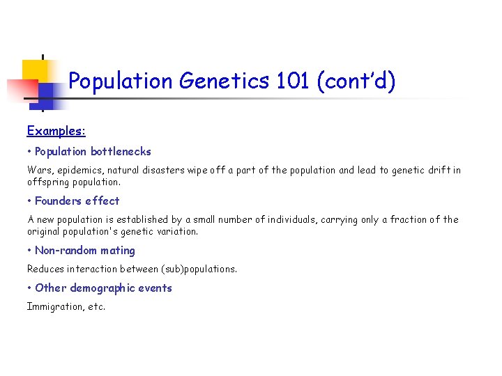
Population Genetics 101 (cont’d) Examples: • Population bottlenecks Wars, epidemics, natural disasters wipe off a part of the population and lead to genetic drift in offspring population. • Founders effect A new population is established by a small number of individuals, carrying only a fraction of the original population's genetic variation. • Non-random mating Reduces interaction between (sub)populations. • Other demographic events Immigration, etc.

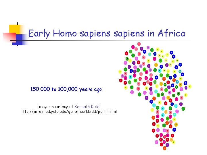
Early Homo sapiens in Africa 150, 000 to 100, 000 years ago Images courtesy of Kenneth Kidd, http: //info. med. yale. edu/genetics/kkidd/point. html

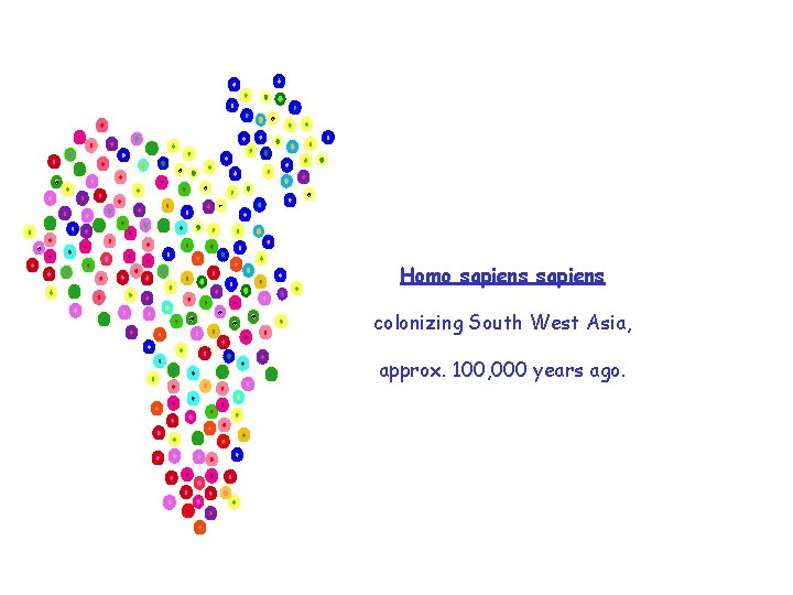
Homo sapiens colonizing South West Asia, approx. 100, 000 years ago.

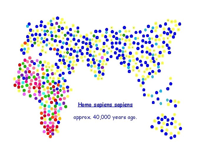
Homo sapiens approx. 40, 000 years ago.

Why study population structure? Ø History of human populations Ø Genealogy Ø Forensics Ø Mapping causative genes for common complex disorders (e. g. diabetes, heart conditions, obesity, etc. )

Why are SNPs really important? Genome Wide Association Studies (GWAS): Locating causative genes for common complex disorders is based on identifying association between affection status and known SNPs. No prior knowledge about the function of the gene(s) or the etiology of the disorder is necessary.

Why are SNPs really important? Genome Wide Association Studies (GWAS): Locating causative genes for common complex disorders is based on identifying association between affection status and known SNPs. No prior knowledge about the function of the gene(s) or the etiology of the disorder is necessary. The subsequent investigation of candidate genes that are in physical proximity with the associated SNPs is the first step towards understanding the etiological pathway of a disorder and designing a drug. Numerous such studies revealed (and will continue to reveal) correlations between genes and diseases.

Recall our objective Develop unsupervised, efficient algorithms for the selection of a small set of SNPs that can be used to Ø capture population structure, and Ø predict individual ancestry. Why? cost efficiency, identification of regions of natural selection. Let’s discuss (briefly) prior work …

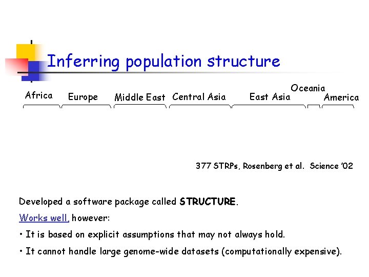
Inferring population structure Africa Europe Middle East Central Asia Oceania East Asia America 377 STRPs, Rosenberg et al. Science ’ 02 Developed a software package called STRUCTURE. Works well, however: • It is based on explicit assumptions that may not always hold. • It cannot handle large genome-wide datasets (computationally expensive).

Selecting ancestry informative markers Existing methods (Fst, Informativeness, δ) Rosenberg et al. Am J Hum Genet ’ 03 Ø Allele frequency based. Ø Require prior knowledge of individual ancestry (supervised). Such knowledge may not be available. (E. g. , populations of complex ancestry, large multi-centered studies of anonymous samples, etc. )

Overview • Basic genetics background • The Singular Value Decomposition (SVD) • The CX decomposition • Selecting Ancestry Informative Markers Ø The Hap. Map data Ø A worldwide set of populations Ø An admixed population

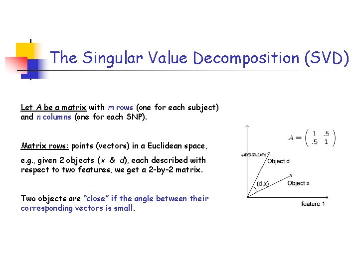
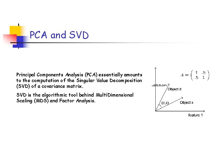
The Singular Value Decomposition (SVD) Let A be a matrix with m rows (one for each subject) and n columns (one for each SNP). Matrix rows: points (vectors) in a Euclidean space, e. g. , given 2 objects (x & d), each described with respect to two features, we get a 2 -by-2 matrix. Two objects are “close” if the angle between their corresponding vectors is small.

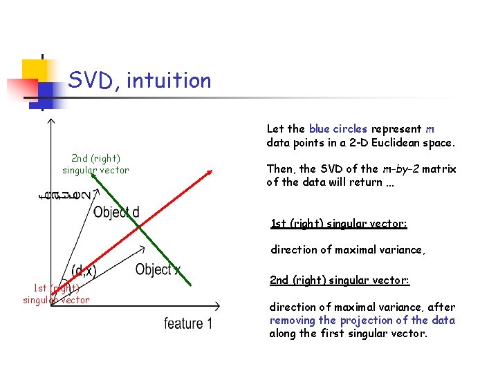
SVD, intuition Let the blue circles represent m data points in a 2 -D Euclidean space. 2 nd (right) singular vector Then, the SVD of the m-by-2 matrix of the data will return … 1 st (right) singular vector: direction of maximal variance, 1 st (right) singular vector 2 nd (right) singular vector: direction of maximal variance, after removing the projection of the data along the first singular vector.

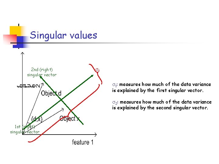
Singular values 2 2 nd (right) singular vector 1: measures how much of the data variance is explained by the first singular vector. 2: measures how much of the data variance is explained by the second singular vector. 1 1 st (right) singular vector

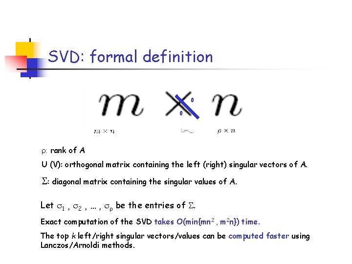
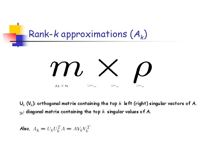
SVD: formal definition 0 0 : rank of A U (V): orthogonal matrix containing the left (right) singular vectors of A. : diagonal matrix containing the singular values of A. Let 1 ¸ 2 ¸ … ¸ be the entries of . Exact computation of the SVD takes O(min{mn 2 , m 2 n}) time. The top k left/right singular vectors/values can be computed faster using Lanczos/Arnoldi methods.

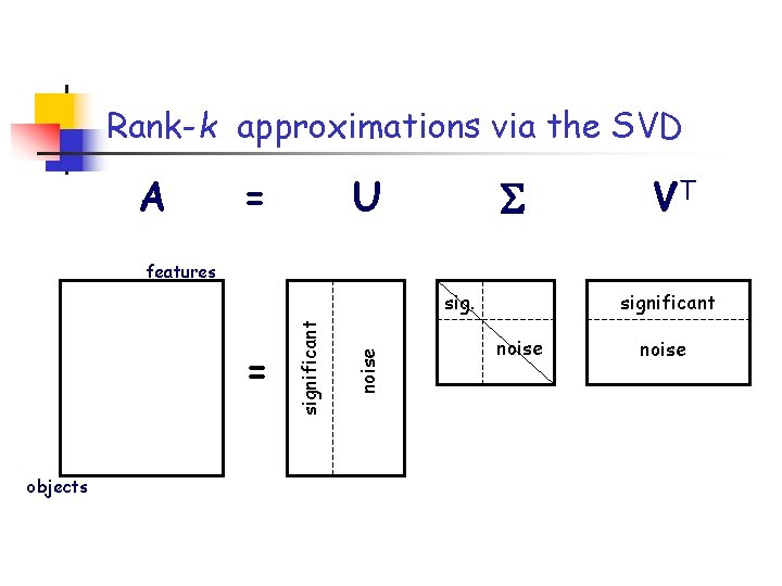
Rank-k approximations via the SVD A = U VT features objects noise = significant noise

Rank-k approximations (Ak) Uk (Vk): orthogonal matrix containing the top k left (right) singular vectors of A. k: diagonal matrix containing the top k singular values of A. Also,

PCA and SVD Principal Components Analysis (PCA) essentially amounts to the computation of the Singular Value Decomposition (SVD) of a covariance matrix. SVD is the algorithmic tool behind Multi. Dimensional Scaling (MDS) and Factor Analysis.

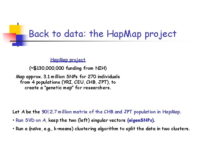
Back to data: the Hap. Map project (~$130, 000 funding from NIH) Map approx. 3. 1 million SNPs for 270 individuals from 4 populations (YRI, CEU, CHB, JPT), to create a “genetic map” for researchers. Let A be the 90£ 2. 7 million matrix of the CHB and JPT population in Hap. Map. • Run SVD on A, keep the two (left) singular vectors (eigen. SNPs). • Run a (naïve, e. g. , k-means) clustering algorithm to split the data in two clusters.

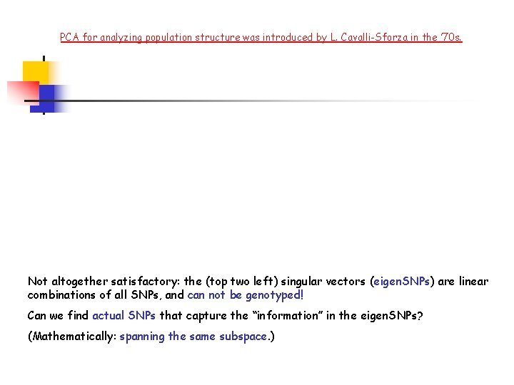
PCA for analyzing population structure was introduced by L. Cavalli-Sforza in the ’ 70 s.

PCA for analyzing population structure was introduced by L. Cavalli-Sforza in the ’ 70 s. Not altogether satisfactory: the (top two left) singular vectors (eigen. SNPs) are linear combinations of all SNPs, and can not be genotyped! Can we find actual SNPs that capture the “information” in the eigen. SNPs? (Mathematically: spanning the same subspace. )

Overview • Basic genetics background • The Singular Value Decomposition (SVD) • The CX decomposition • Selecting Ancestry Informative Markers Ø The Hap. Map data Ø A worldwide set of populations Ø An admixed population

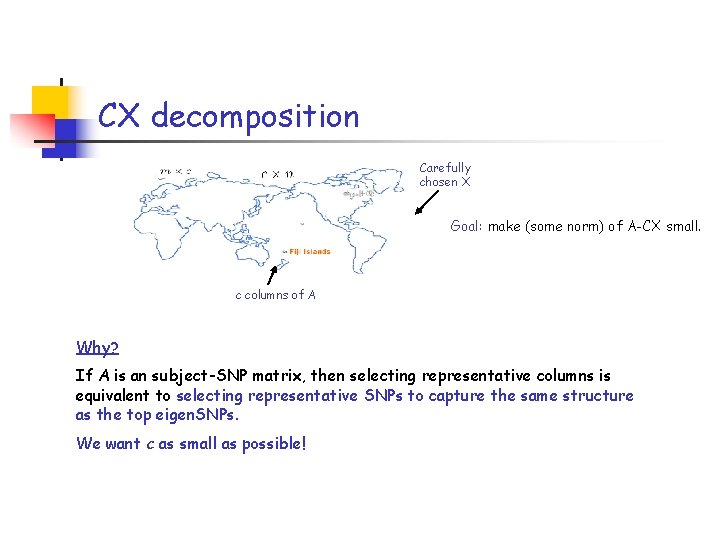
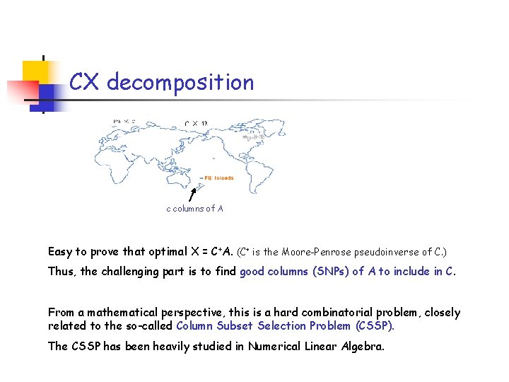
CX decomposition Carefully chosen X Goal: make (some norm) of A-CX small. c columns of A Why? If A is an subject-SNP matrix, then selecting representative columns is equivalent to selecting representative SNPs to capture the same structure as the top eigen. SNPs. We want c as small as possible!

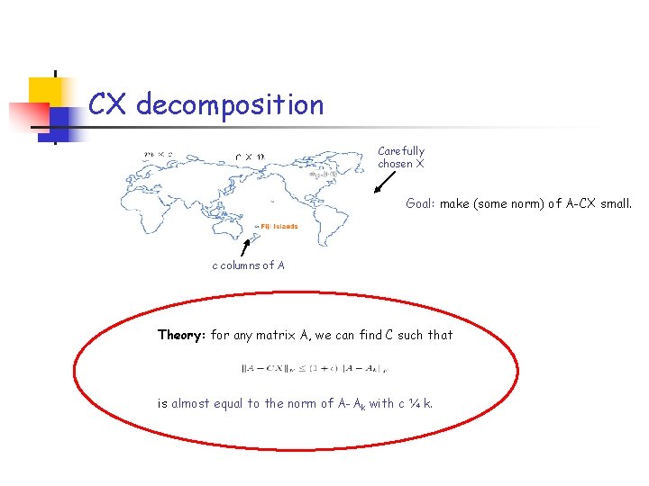
CX decomposition Carefully chosen X Goal: make (some norm) of A-CX small. c columns of A Theory: for any matrix A, we can find C such that is almost equal to the norm of A-Ak with c ¼ k.

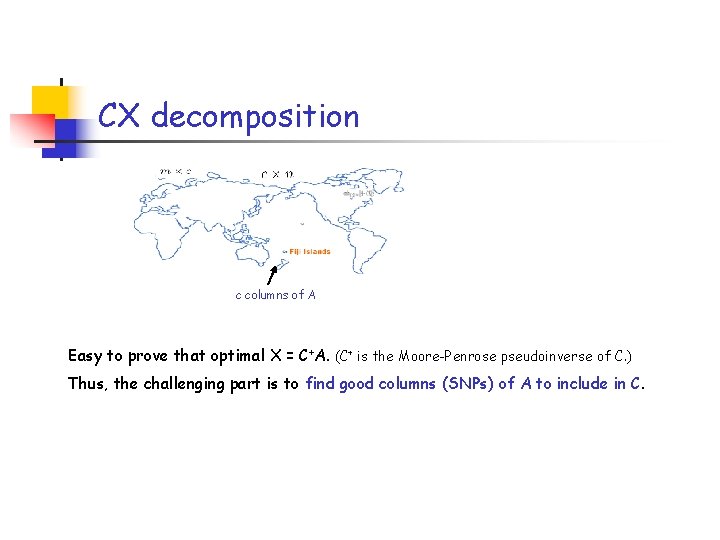
CX decomposition c columns of A Easy to prove that optimal X = C+A. (C+ is the Moore-Penrose pseudoinverse of C. ) Thus, the challenging part is to find good columns (SNPs) of A to include in C.

CX decomposition c columns of A Easy to prove that optimal X = C+A. (C+ is the Moore-Penrose pseudoinverse of C. ) Thus, the challenging part is to find good columns (SNPs) of A to include in C. From a mathematical perspective, this is a hard combinatorial problem, closely related to the so-called Column Subset Selection Problem (CSSP). The CSSP has been heavily studied in Numerical Linear Algebra.

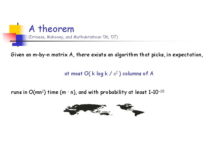
A theorem (Drineas, Mahoney, and Muthukrishnan ’ 06, ’ 07) Given an m-by-n matrix A, there exists an algorithm that picks, in expectation, at most O( k log k / 2 ) columns of A runs in O(mn 2) time (m · n), and with probability at least 1 -10 -20

The CX algorithm Input: m-by-n matrix A, integer k Output: C, the matrix consisting of the selected columns CX algorithm • Compute probabilities pj summing to 1 • Let c = O(k log k / 2) • For each j = 1, 2, …, n, pick the j-th column of A with probability min{1, cpj} • Let C be the matrix consisting of the chosen columns (C has – in expectation – at most c columns)

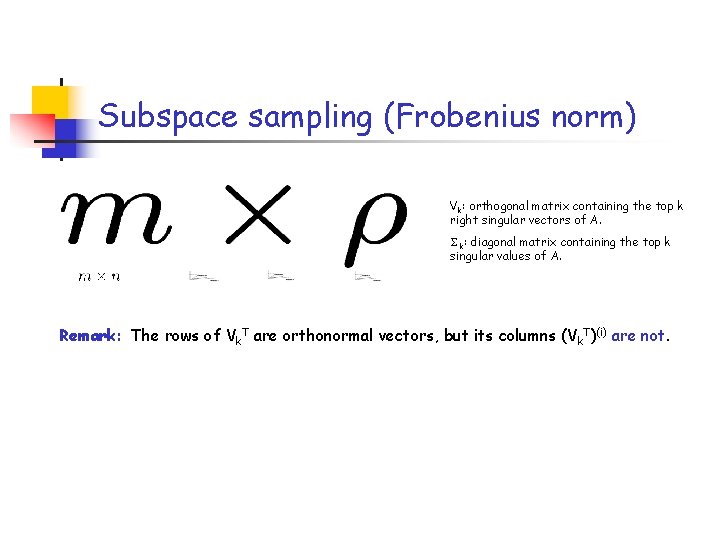
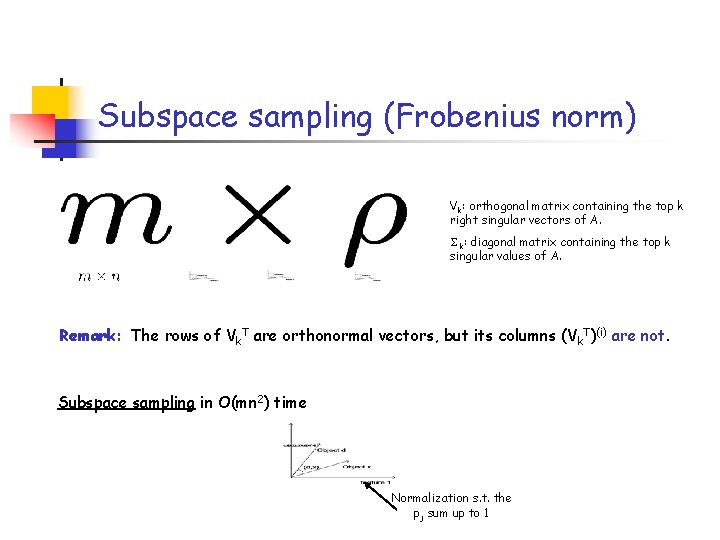
Subspace sampling (Frobenius norm) Vk: orthogonal matrix containing the top k right singular vectors of A. k: diagonal matrix containing the top k singular values of A. Remark: The rows of Vk. T are orthonormal vectors, but its columns (Vk. T)(i) are not.

Subspace sampling (Frobenius norm) Vk: orthogonal matrix containing the top k right singular vectors of A. k: diagonal matrix containing the top k singular values of A. Remark: The rows of Vk. T are orthonormal vectors, but its columns (Vk. T)(i) are not. Subspace sampling in O(mn 2) time Normalization s. t. the pj sum up to 1

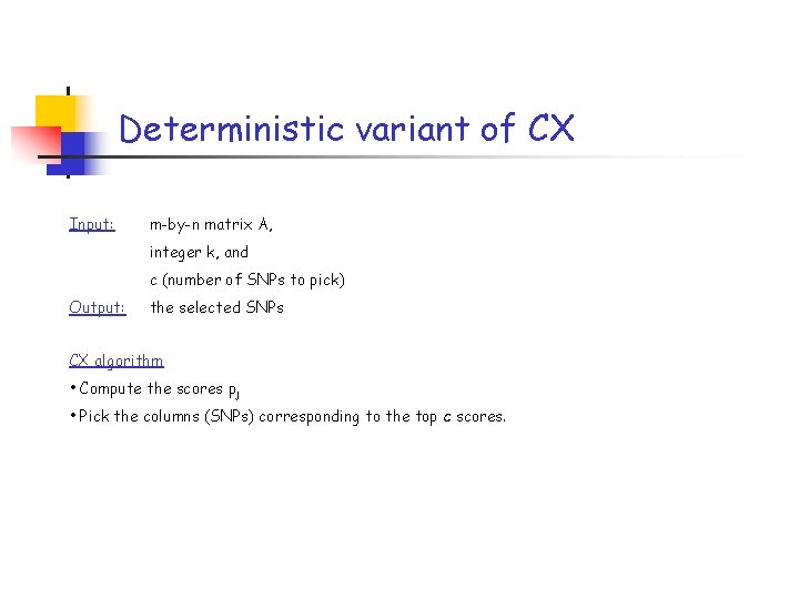
Deterministic variant of CX Input: m-by-n matrix A, integer k, and c (number of SNPs to pick) Output: the selected SNPs CX algorithm • Compute the scores pj • Pick the columns (SNPs) corresponding to the top c scores.

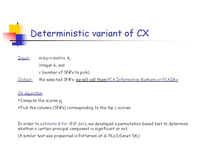
Deterministic variant of CX Input: m-by-n matrix A, integer k, and c (number of SNPs to pick) Output: the selected SNPs: we will call them PCA Informative Markers or PCAIMs CX algorithm • Compute the scores pj • Pick the columns (SNPs) corresponding to the top c scores. In order to estimate k for SNP data, we developed a permutation-based test to determine whether a certain principal component is significant or not. (A similar test was presented in Patterson et al. PLo. S Genet ’ 06. )

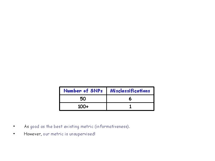
Number of SNPs Misclassifications 50 6 100+ 1 • As good as the best existing metric (informativeness). • However, our metric is unsupervised!

Overview • Basic genetics background • The Singular Value Decomposition (SVD) • The CX decomposition • Selecting Ancestry Informative Markers Ø The Hap. Map data Ø A worldwide set of populations Ø An admixed population

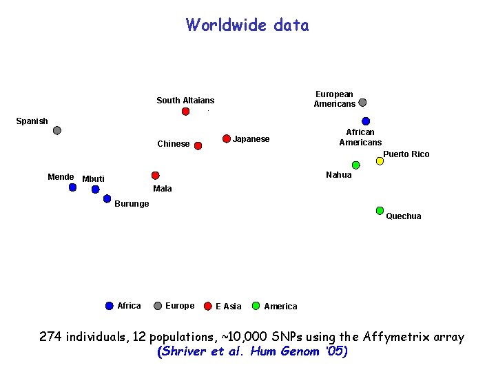
Worldwide data European Americans South Altaians - Spanish Chinese Japanese African Americans Puerto Rico Mende Nahua Mbuti Mala Burunge Quechua Africa Europe E Asia America 274 individuals, 12 populations, ~10, 000 SNPs using the Affymetrix array (Shriver et al. Hum Genom ‘ 05)

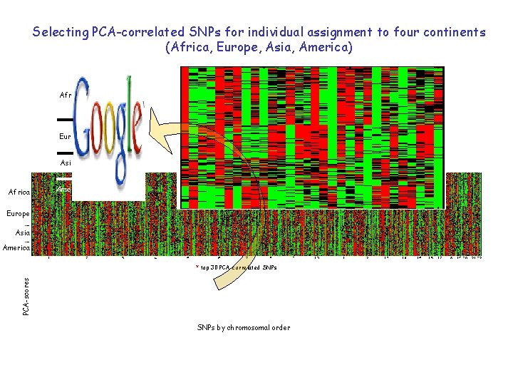
Selecting PCA-correlated SNPs for individual assignment to four continents (Africa, Europe, Asia, America) Afr Eur Asi Africa Ame Europe Asia America PCA-scores * top 30 PCA-correlated SNPs by chromosomal order

Correlation coefficient between true and predicted membership of an individual to a particular geographic continent. (Use a subset of SNPs, cluster the individuals using k-means. )

Cross-validation on Hap. Map data

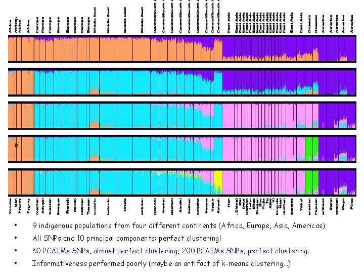
A B • 9 indigenous populations from four different continents (Africa, Europe, Asia, Americas) • All SNPs and 10 principal components: perfect clustering! • 50 PCAIMs SNPs, almost perfect clustering; 200 PCAIMs SNPs, perfect clustering. • Informativeness performed poorly (maybe an artifact of k-means clustering…)

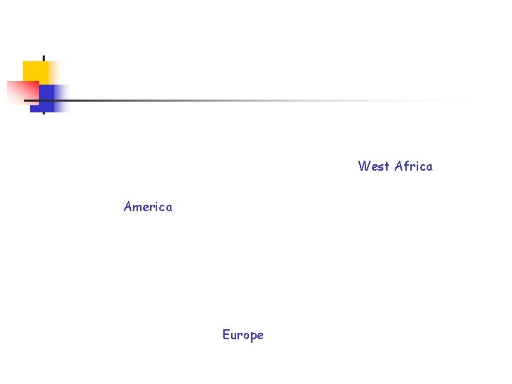
Admixed populations Two (independent) Puerto Rican datasets, two major axes of variation: • Dataset A: 192 individuals, ~7, 000 SNPs • Dataset B: 30 individuals, same ~7, 000 SNP • European - West African axis of variation • Native American axis of variation

West Africa America Europe

Europe-Africa axis of variation Europe Ancestry coefficient: location of the individual in the Europe - Africa axis. Africa

Predicting ancestry using PCAIMs

Predicting ancestry using PCAIMs

Cross-validation on Puerto-Rican dataset B

Conclusions Ø Using linear algebraic techniques (e. g. , matrix decompositions) we selected markers that capture population structure. Ø Our technique requires no prior assumptions and builds upon the power of SVD to identify population structure in various settings, including admixed populations. Ø Prior theoretical work and mathematical understanding of the underlying problem was fundamental in designing our algorithm!

Acknowledgements Collaborators Students P. Paschou, Democritus University, Greece E. Ziv, UCSF E. Burchard, UCSF M. W. Mahoney, Yahoo! Research K. K. Kidd, Yale University M. Shriver, Penn State R. Krauss, Oakland Research Institute Asif Javed, RPI Jamey Lewis, RPI Funding NSF CAREER award to Petros Drineas NIH U 19 AG 23122 and K 22 CA 109351 Breast Cancer Research Program grant to E. Ziv Hellenic Endocrine Society Research grant award to P. Paschou Ref: Paschou, Elad, Burchard, …, Mahoney, and Drineas (2007) PLo. S Genetics, 3: e 160