Hypothesis Testing Goal Make statements regarding unknown population

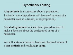
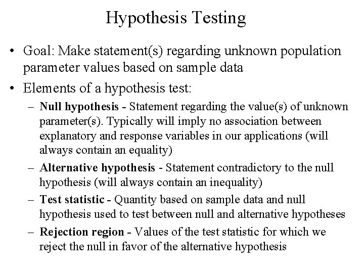
Hypothesis Testing • Goal: Make statement(s) regarding unknown population parameter values based on sample data • Elements of a hypothesis test: – Null hypothesis - Statement regarding the value(s) of unknown parameter(s). Typically will imply no association between explanatory and response variables in our applications (will always contain an equality) – Alternative hypothesis - Statement contradictory to the null hypothesis (will always contain an inequality) – Test statistic - Quantity based on sample data and null hypothesis used to test between null and alternative hypotheses – Rejection region - Values of the test statistic for which we reject the null in favor of the alternative hypothesis

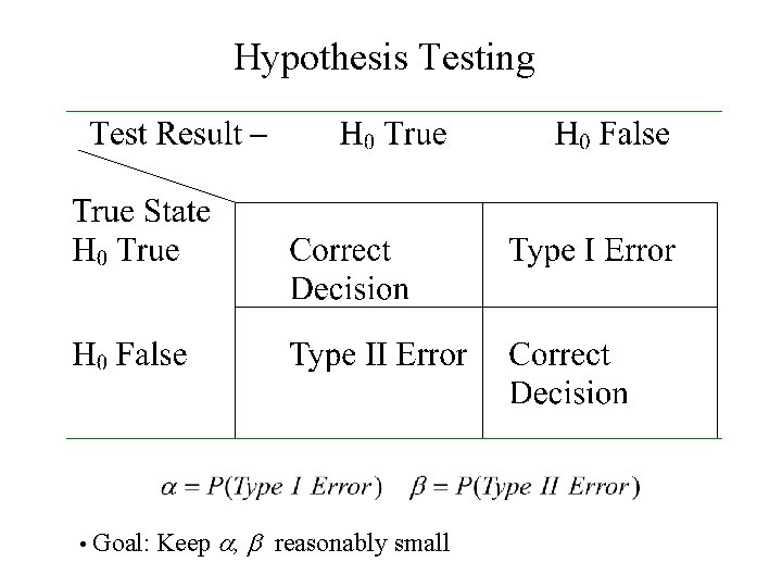
Hypothesis Testing • Goal: Keep a, b reasonably small

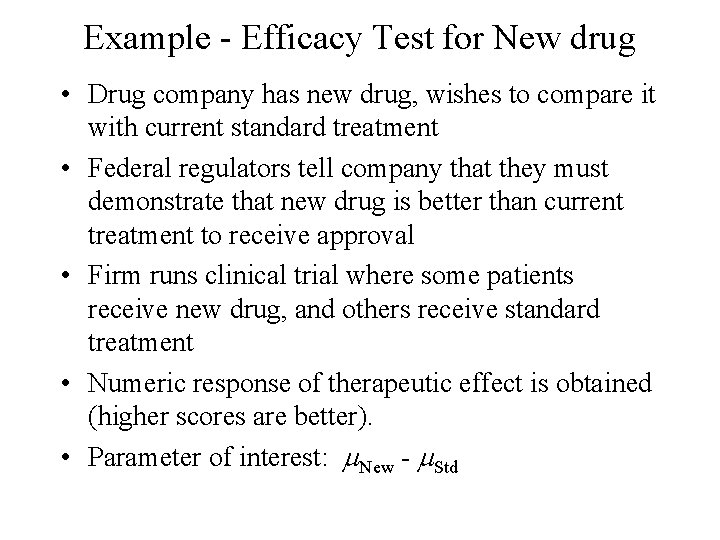
Example - Efficacy Test for New drug • Drug company has new drug, wishes to compare it with current standard treatment • Federal regulators tell company that they must demonstrate that new drug is better than current treatment to receive approval • Firm runs clinical trial where some patients receive new drug, and others receive standard treatment • Numeric response of therapeutic effect is obtained (higher scores are better). • Parameter of interest: m. New - m. Std

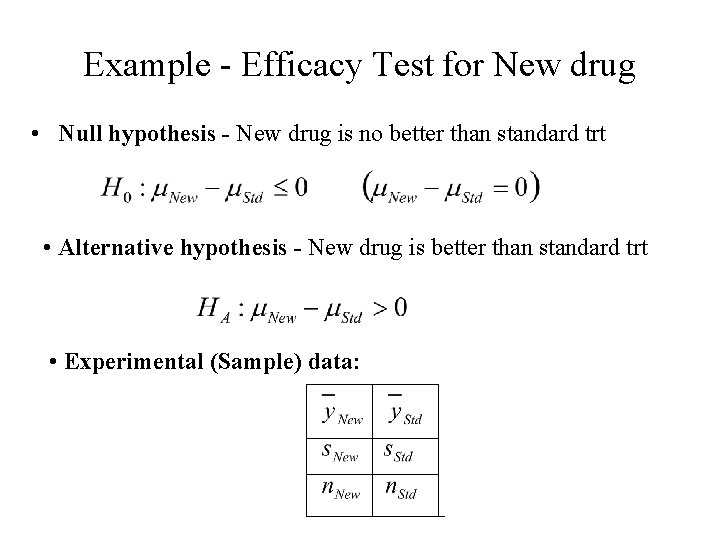
Example - Efficacy Test for New drug • Null hypothesis - New drug is no better than standard trt • Alternative hypothesis - New drug is better than standard trt • Experimental (Sample) data:

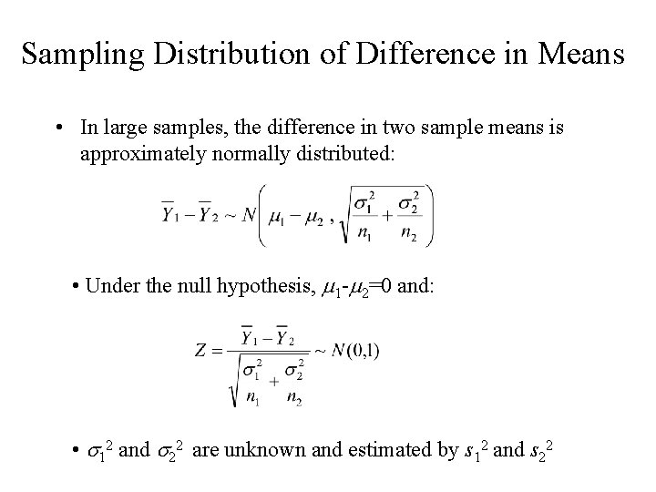
Sampling Distribution of Difference in Means • In large samples, the difference in two sample means is approximately normally distributed: • Under the null hypothesis, m 1 -m 2=0 and: • s 12 and s 22 are unknown and estimated by s 12 and s 22

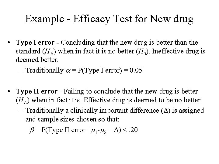
Example - Efficacy Test for New drug • Type I error - Concluding that the new drug is better than the standard (HA) when in fact it is no better (H 0). Ineffective drug is deemed better. – Traditionally a = P(Type I error) = 0. 05 • Type II error - Failing to conclude that the new drug is better (HA) when in fact it is. Effective drug is deemed to be no better. – Traditionally a clinically important difference (D) is assigned and sample sizes chosen so that: b = P(Type II error | m 1 -m 2 = D) . 20

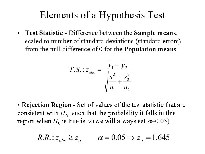
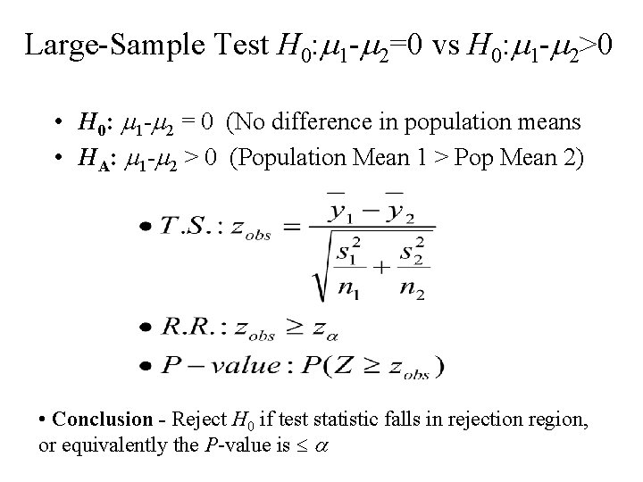
Elements of a Hypothesis Test • Test Statistic - Difference between the Sample means, scaled to number of standard deviations (standard errors) from the null difference of 0 for the Population means: • Rejection Region - Set of values of the test statistic that are consistent with HA, such that the probability it falls in this region when H 0 is true is a (we will always set a=0. 05)

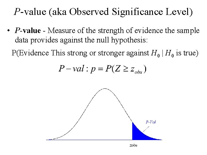
P-value (aka Observed Significance Level) • P-value - Measure of the strength of evidence the sample data provides against the null hypothesis: P(Evidence This strong or stronger against H 0 | H 0 is true)

Large-Sample Test H 0: m 1 -m 2=0 vs H 0: m 1 -m 2>0 • H 0: m 1 -m 2 = 0 (No difference in population means • HA: m 1 -m 2 > 0 (Population Mean 1 > Pop Mean 2) • Conclusion - Reject H 0 if test statistic falls in rejection region, or equivalently the P-value is a

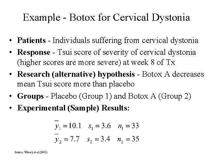
Example - Botox for Cervical Dystonia • Patients - Individuals suffering from cervical dystonia • Response - Tsui score of severity of cervical dystonia (higher scores are more severe) at week 8 of Tx • Research (alternative) hypothesis - Botox A decreases mean Tsui score more than placebo • Groups - Placebo (Group 1) and Botox A (Group 2) • Experimental (Sample) Results: Source: Wissel, et al (2001)

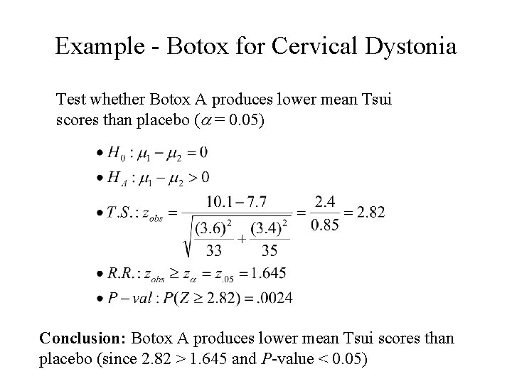
Example - Botox for Cervical Dystonia Test whether Botox A produces lower mean Tsui scores than placebo (a = 0. 05) Conclusion: Botox A produces lower mean Tsui scores than placebo (since 2. 82 > 1. 645 and P-value < 0. 05)

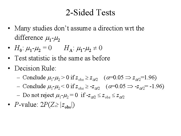
2 -Sided Tests • Many studies don’t assume a direction wrt the difference m 1 -m 2 • H 0: m 1 -m 2 = 0 HA: m 1 -m 2 0 • Test statistic is the same as before • Decision Rule: – Conclude m 1 -m 2 > 0 if zobs za/2 (a=0. 05 za/2=1. 96) – Conclude m 1 -m 2 < 0 if zobs -za/2 (a=0. 05 -za/2= -1. 96) – Do not reject m 1 -m 2 = 0 if -za/2 zobs za/2 • P-value: 2 P(Z |zobs|)

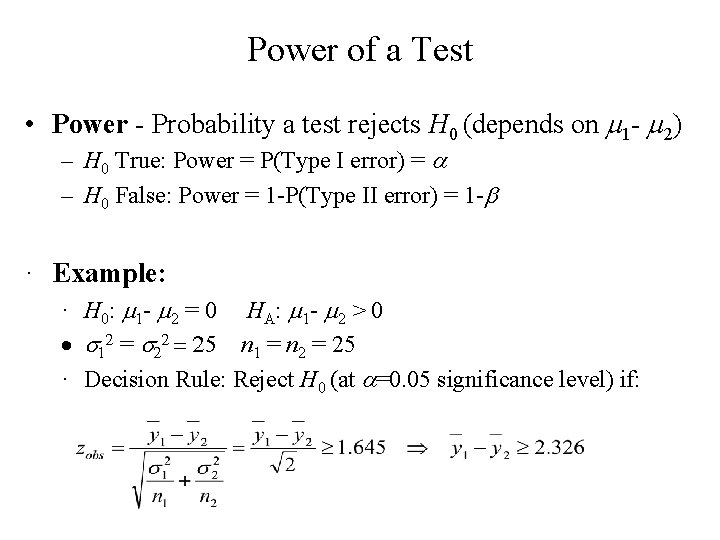
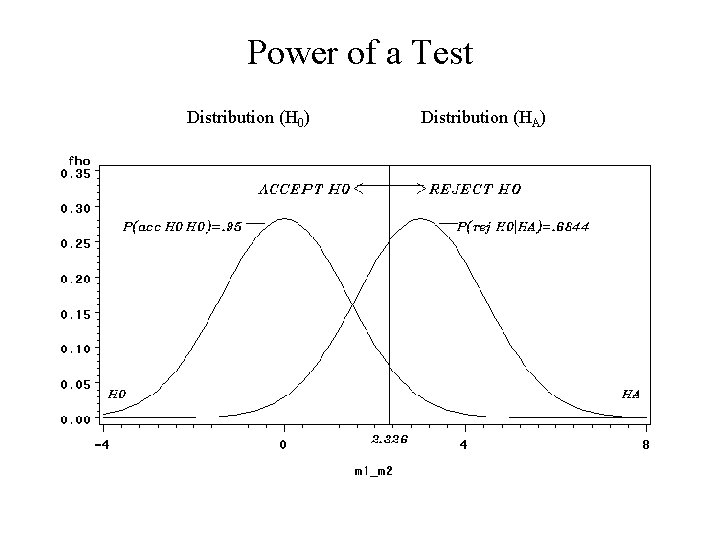
Power of a Test • Power - Probability a test rejects H 0 (depends on m 1 - m 2) – H 0 True: Power = P(Type I error) = a – H 0 False: Power = 1 -P(Type II error) = 1 -b · Example: · H 0: m 1 - m 2 = 0 HA: m 1 - m 2 > 0 · s 12 = s 22 = 25 n 1 = n 2 = 25 · Decision Rule: Reject H 0 (at a=0. 05 significance level) if:

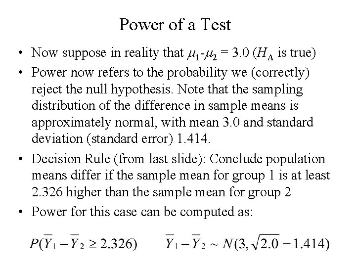
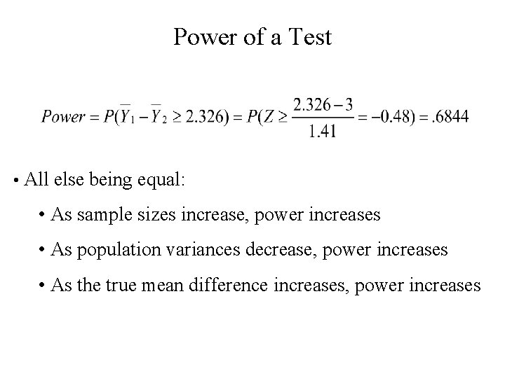
Power of a Test • Now suppose in reality that m 1 -m 2 = 3. 0 (HA is true) • Power now refers to the probability we (correctly) reject the null hypothesis. Note that the sampling distribution of the difference in sample means is approximately normal, with mean 3. 0 and standard deviation (standard error) 1. 414. • Decision Rule (from last slide): Conclude population means differ if the sample mean for group 1 is at least 2. 326 higher than the sample mean for group 2 • Power for this case can be computed as:

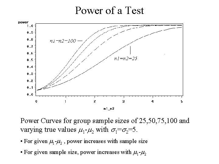
Power of a Test • All else being equal: • As sample sizes increase, power increases • As population variances decrease, power increases • As the true mean difference increases, power increases

Power of a Test Distribution (H 0) Distribution (HA)

Power of a Test Power Curves for group sample sizes of 25, 50, 75, 100 and varying true values m 1 -m 2 with s 1=s 2=5. • For given m 1 -m 2 , power increases with sample size • For given sample size, power increases with m 1 -m 2

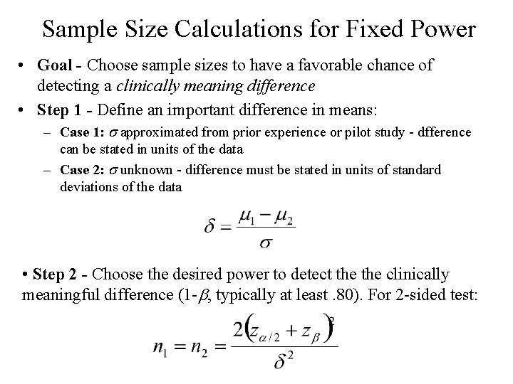
Sample Size Calculations for Fixed Power • Goal - Choose sample sizes to have a favorable chance of detecting a clinically meaning difference • Step 1 - Define an important difference in means: – Case 1: s approximated from prior experience or pilot study - dfference can be stated in units of the data – Case 2: s unknown - difference must be stated in units of standard deviations of the data • Step 2 - Choose the desired power to detect the clinically meaningful difference (1 -b, typically at least. 80). For 2 -sided test:

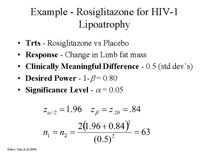
Example - Rosiglitazone for HIV-1 Lipoatrophy • • • Trts - Rosiglitazone vs Placebo Response - Change in Limb fat mass Clinically Meaningful Difference - 0. 5 (std dev’s) Desired Power - 1 -b = 0. 80 Significance Level - a = 0. 05 Source: Carr, et al (2004)

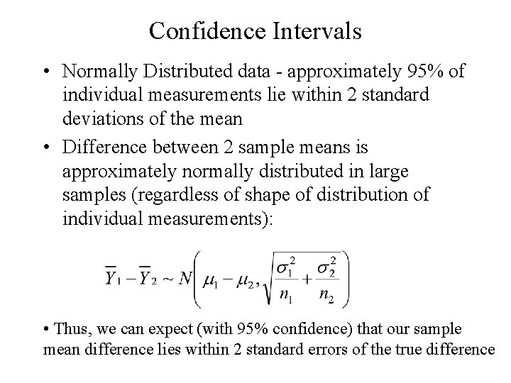
Confidence Intervals • Normally Distributed data - approximately 95% of individual measurements lie within 2 standard deviations of the mean • Difference between 2 sample means is approximately normally distributed in large samples (regardless of shape of distribution of individual measurements): • Thus, we can expect (with 95% confidence) that our sample mean difference lies within 2 standard errors of the true difference

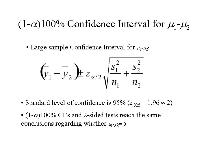
(1 -a)100% Confidence Interval for m 1 -m 2 • Large sample Confidence Interval for m 1 -m 2: • Standard level of confidence is 95% (z. 025 = 1. 96 2) • (1 -a)100% CI’s and 2 -sided tests reach the same conclusions regarding whether m 1 -m 2= 0

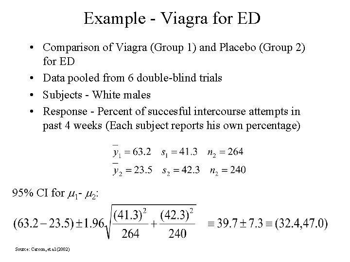
Example - Viagra for ED • Comparison of Viagra (Group 1) and Placebo (Group 2) for ED • Data pooled from 6 double-blind trials • Subjects - White males • Response - Percent of succesful intercourse attempts in past 4 weeks (Each subject reports his own percentage) 95% CI for m 1 - m 2: Source: Carson, et al (2002)