How to Think Algorithmically in Parallel Uzi Vishkin

How to Think Algorithmically in Parallel? Uzi Vishkin

Who should produce the parallel code? Choices [state-of-the-art compiler research perspective] • Programmer only Thanks: Prof. Barua – Writing parallel code is tedious. – Good at ‘seeing parallelism’, esp. irregular parallelism. – But are bad at seeing locality and granularity considerations. • Have poor intuitions about compiler transformations. • Compiler only – Can see regular parallelism, but not irregular parallelism. – Great at doing compiler transformations to improve parallelism, granularity and locality. Hybrid solution: Programmer specifies high-level parallelism, but little else. Compiler does the rest. (My) Broader questions Goals: Where will the algorithms come from? • Ease of programming Is today’s HW good enough? – Declarative programming This course relevant for all 3 questions

Serial RAM Step: 1 op (memory/etc). PRAM (Parallel Random-Access Model) Step: many ops. Serial doctrine algorithm What could I do in parallel at each step assuming unlimited hardware # # ops. . time = #ops . . ops Natural (parallel) . . time << #ops 1979 - : THEORY figure out how to think algorithmically in parallel

Flavor of parallelism Exchange Problem Replace A and B. Ex. A=2, B=5 A=5, B=2. Serial Alg: X: =A; A: =B; B: =X. 3 Ops. 3 Steps. Space 1. Fewer steps (FS): X: =A B: =X Y: =B A: =Y 4 ops. 2 Steps. Space 2. Array Exchange Problem Given A[1. . n] & B[1. . n], replace A(i) and B(i), i=1. . n. Serial Alg: For i=1 to n do X: =A(i); A(i): =B(i); B(i): =X /*serial replace 3 n Ops. 3 n Steps. Space 1. Par Alg 1: For i=1 to n pardo X(i): =A(i); A(i): =B(i); B(i): =X(i) /*serial replace in parallel 3 n Ops. 3 Steps. Space n. Par Alg 2: For i=1 to n pardo X(i): =A(i) B(i): =X(i) Y(i): =B(i) A(i): =Y(i) /*FS in parallel 4 n Ops. 2 Steps. Space 2 n. Discussion - Parallelism requires extra space (memory). - Par Alg 1 clearly faster than Serial Alg. - Is Par Alg 2 preferred to Par Alg 1?

Snapshot: XMT High-level language XMTC: Single-program multiple-data (SPMD) extension of standard C. Includes Spawn and PS - a multi-operand instruction. Short (not OS) threads. Cartoon Spawn creates threads; a thread progresses at its own speed and expires at its Join. Synchronization: only at the Joins. So, virtual threads avoid busy-waits by expiring. New: Independence of order semantics (IOS). Array Exchange. Pseudo-code for Par Alg 1 Spawn(1, n){ X($): =A($); A($): =B($); B($): =X($) }

Example of Parallel algorithm Breadth-First-Search (BFS)

(i) “Concurrently” as in natural BFS: only change to serial algorithm (ii) Defies “decomposition”/”partition” Parallel complexity W = ~(|V| + |E|) T = ~d, the number of layers Average parallelism = ~W/T Mental effort 1. Sometimes easier than serial 2. Within common denominator of other parallel approaches. In fact, much easier

XMT project at UMD Algorithms PRAM-On-Chip HW Prototypes PRAM parallel algorithmic theory. 64 -core, 75 MHz FPGA of XMT (Explicit Multi-Threaded) architecture “Natural selection”. Latent, SPAA 98. . CF 08 though not widespread, knowledgebase ICE/Work. Depth Conjecture SV 82: The rest (full PRAM algorithm) 128 -core intercon. network just a matter of skill IBM 90 nm: 9 mm. X 5 mm, 400 MHz [Hot. I 07] Fund Lots of evidence that “work-depth” work on asynch NOCS’ 10 works. Used as framework in main PRAM algorithms texts: • FPGA design ASIC Ja. Ja 92, KKT 01 • IBM 90 nm: 10 mm. X 10 mm programming & workflow • Stable compiler. Architecture scales to 1000+ cores on-chip

Software release Allows to use your own computer for programming on an XMT environment and experimenting with it, including: (i)Cycle-accurate simulator of the XMT machine (ii)Compiler from XMTC to that machine Also provided, extensive material for teaching or self-studying parallelism, including (i)Tutorial + manual for XMTC (150 pages) (ii)Classnotes on parallel algorithms (100 pages) (iii)Video recording of 9/15/07 HS tutorial (300 minutes)

Parallel Random-Access Machine/Model PRAM: n synchronous processors all having unit time access to a shared memory. Each processor has also a local memory. At each time unit, a processor can: 1. write into the shared memory (i. e. , copy one of its local memory registers into a shared memory cell), 2. read into shared memory (i. e. , copy a shared memory cell into one of its local memory registers ), or 3. do some computation with respect to its local memory.

pardo programming construct - for Pi , 1 ≤ i ≤ n pardo - A(i) : = B(i) This means The following n operations are performed concurrently: processor P 1 assigns B(1) into A(1), processor P 2 assigns B(2) into A(2), …. Modeling read&write conflicts to the same shared memory location Most common are: - exclusive-read exclusive-write (EREW) PRAM: no simultaneous access by more than one processor to the same memory location for read or write purposes - concurrent-read exclusive-write (CREW) PRAM: concurrent access for reads but not for writes - concurrent-read concurrent-write (CRCW allows concurrent access for both reads and writes. We shall assume that in a concurrent-write model, an arbitrary processor among the processors attempting to write into a common memory location, succeeds. This is called the Arbitrary CRCW rule. There are two alternative CRCW rules: (i) Priority CRCW: the smallest numbered, among the processors attempting to write into a common memory location, actually succeeds. (ii) Common CRCW: allows concurrent writes only when all the processors attempting to write into a common memory location are trying to write the same value.

Example of a PRAM algorithm: The summation problem Input An array A = A(1). . . A(n) of n numbers. The problem is to compute A(1) +. . . + A(n). The summation algorithm works in rounds. Each round: add, in parallel, pairs of elements: add each odd-numbered element and its successive even-numbered element. If n = 8, outcome of 1 st round is: A(1) + A(2), A(3) + A(4), A(5) + A(6), A(7) + A(8) Outcome of 2 nd round: A(1) + A(2) + A(3) + A(4), A(5) + A(6) + A(7) + A(8) and the outcome of 3 rd (and last) round: A(1) + A(2) + A(3) + A(4) + A(5) + A(6) + A(7) + A(8) B – 2 -dimensional array (whose entries are B(h, i), 0 ≤ h ≤ log n and 1 ≤ i ≤ n/2 h) used to store all intermediate steps of the computation (base of logarithm: 2). For simplicity, assume n = 2 k for some integer k. ALGORITHM 1 (Summation) Algorithm 1 uses p = n processors. 1. for Pi , 1 ≤ i ≤ n pardo Line 2 takes one round, 2. B(0, i) : = A(i) Line 3 defines a loop taking 3. for h : = 1 to log n do log n rounds 4. if i ≤ n/2 h 5. then B(h, i) : = B(h − 1, 2 i − 1) + B(h − 1, 2 i) Line 7 takes one round. 6. else stay idle 7. for i = 1: output B(log n, 1); for i > 1: stay idle

Summation on an n = 8 processor PRAM Again Algorithm 1 uses p = n processors. Line 2 takes one round, line 3 defines a loop taking log n rounds, and line 7 takes one round. Since each round takes constant time, Algorithm 1 runs in O(log n) time. [When you see O (“big Oh”), think “proportional to”. ] S So, o an algorithm in the PRAM model is, presented in terms of a sequence of parallel time a units (or “rounds”, or “pulses”); we allow n p instructions to be performed at each time a unit, one per processor; this means that l a time unit consists of a sequence of exactly p instructions to be performed g concurrently. o r i t

2 drawbacks to PRAM mode: (i) Does not reveal how the algorithm will run on PRAMs with different number of processors; e. g. , to what extent will more processors speed the computation, or fewer processors slow it? (ii) Fully specifying the allocation of instructions to processors requires a level of detail which might be unnecessary (a compiler may be able to extract from lesser detail) Work-Depth presentation of algorithms Alternative model and presentation mode. Work-Depth algorithms are also presented as a sequence of parallel time units (or “rounds”, or “pulses”); however, each time unit consists of a sequence of instructions to be performed concurrently; the sequence of instructions may include any number.

WD presentation of the summation example “Greedy-parallelism”: At each point in time, the (WD) summation algorithm seeks to break the problem into as many pair wise additions as possible, or, in other words, into the largest possible number of independent tasks that can performed concurrently. ALGORITHM 2 (WD-Summation) 1. for i , 1 ≤ i ≤ n pardo 2. B(0, i) : = A(i) 3. for h : = 1 to log n 4. for i , 1 ≤ i ≤ n/2 h pardo 5. B(h, i) : = B(h − 1, 2 i − 1) + B(h − 1, 2 i) 6. for i = 1 pardo output B(log n, 1) The 1 st round of the algorithm (lines 1&2) has n operations. The 2 nd round (lines 4&5 for h = 1) has n/2 operations. The 3 rd round (lines 4&5 for h = 2) has n/4 operations. In general, the k-th round of the algorithm, 1 ≤ k ≤ log n + 1, has n/2 k-1 operations and round log n +2 (line 6) has one more operation (use of a pardo instruction in line 6 is somewhat artificial). The total number of operations is 2 n and the time is log n + 2. We will use this information in the corollary below. The next theorem demonstrates that the WD presentation mode does not suffer from the same drawbacks as the standard PRAM mode, and that every algorithm in the WD mode can be automatically translated into a PRAM algorithm.

The WD-presentation sufficiency Theorem Consider an algorithm in the WD mode that takes a total of x = x(n) elementary operations and d = d(n) time. The algorithm can be implemented by any p = p(n)-processor PRAM within O(x/p + d) time, using the same concurrent-write convention as in the WD presentation. [i. e. , 5 theorems: EREW, Common/Arbitrary/Priority CRCW] Proof xi - # instructions at round i. [x 1+x 2+. . +xd = x] p processors can simulate xi instructions in �xi/p� ≤ xi/p + 1 time units. See next slide. Demonstration in Algorithm 2’ shows why you don’t want to leave this to a programmer. Formally: first reads, then writes. Theorem follows, since �x 1/p�+�x 2/p�+. . +�xd/p� ≤ (x 1/p +1)+. . +(xd/p +1) ≤ x/p + d

Round-robin emulation of y concurrent instructions by p processors in �y/p�rounds. In each of the first �y/p�− 1 rounds, p instructions are emulated for a total of z = p(�y/p�− 1) instructions. In round �y/p�, the remaining y − z instructions are emulated, each by a processor, while the remaining w − y processor stay idle, where w = p�y/p�

Corollary for summation example Algorithm 2 would run in O(n/p + log n) time on a p-processor PRAM. For p ≤ n/ log n, this implies O(n/p) time. Later called both optimal speedup & linear speedup For p ≥ n/ log n: O(log n) time. Since no concurrent reads or writes pprocessor EREW PRAM algorithm.

ALGORITHM 2’ (Summation on a p-processor PRAM) 1. for Pi , 1 ≤ i ≤ p pardo 2. for j : = 1 to �n/p�− 1 do B(0, i + (j − 1)p) : = A(i + (j − 1)p) 3. for i , 1 ≤ i ≤ n − (�n/p�− 1)p B(0, i + (�n/p�− 1)p) : = A(i + (�n/p�− 1)p) - for i , n − (�n/p�− 1)p ≤ i ≤ p stay idle 4. for h : = 1 to log n 5. for j : = 1 to �n/(2 hp)�− 1 do (*an instruction j : = 1 to 0 do means: “do nothing”*) B(h, i+(j − 1)p) : = B(h− 1, 2(i+(j − 1)p)− 1) + B(h− 1, 2(i+(j − 1)p)) 6. for i , 1 ≤ i ≤ n − (�n/(2 hp)�− 1)p B(h, i + (�n/(2 hp)�− 1)p) : = B(h − 1, 2(i + (�n/(2 hp)�− 1)p) − 1) + B(h − 1, 2(i + (�n/(2 hp)�− 1)p)) for i , n − (�n/(2 hp)�− 1)p ≤ i ≤ p stay idle 7. for i = 1 output B(log n, 1); for i > 1 stay idle Nothing more than plugging in the above proof. Main point of this slide: compare to Algorithm 2 and decide, which one you like better But is WD mode as easy as it gets? Hold on…Key question for this presentation

Measuring the performance of parallel algorithms A problem. Input size: n. A parallel algorithm in WD mode. Worst case time: T(n); work: W(n). 4 alternative ways to measure performance: 1. W(n) operations and T(n) time. 2. P(n) = W(n)/T(n) processors and T(n) time (on a PRAM). 3. W(n)/p time using any number of p ≤ W(n)/T(n) processors (on a PRAM). 4. W(n)/p + T(n) time using any number of p processors (on a PRAM). Exercise 1: The above four ways for measuring performance of a parallel algorithms form six pairs. Prove that the pairs are all asymptotically equivalent.

Goals for Designers of Parallel Algorithms Suppose 2 parallel algorithms for same problem: 1. W 1(n) operations in T 1(n) time. 2. W 2(n) operations, T 2(n) time. General guideline: algorithm 1 more efficient than algorithm 2 if W 1(n) = o(W 2(n)), regardless of T 1(n) and T 2(n); if W 1(n) and W 2(n) grow asymptotically the same, then algorithm 1 is considered more efficient if T 1(n) = o(T 2(n)). Good reasons for avoiding strict formal definition—only guidelines Example W 1(n)=O(n), T 1(n)=O(n); W 2(n)=O(n log n), T 2(n)=O(log n) Which algorithm is more efficient? Algorithm 1: less work. Algorithm 2: much faster. In this case, both algorithms are probably interesting. Imagine two users, each interested in different input sizes and in different target machines (different # processors). For one user Algorithm 1 faster. For second user Algorithm 2 faster. Known unresolved issues with asymptotic worst-case analysis.

Nicknaming speedups Suppose T(n) best possible worst case time upper bound on serial algorithm for an input of length n for some problem. (T(n) is serial time complexity for problem. ) Let W(n) and Tpar(n) be work and time bounds of a parallel algorithm for same problem. The parallel algorithm is work-optimal, if W(n) grows asymptotically the same as T(n). A work-optimal parallel algorithm is work-time-optimal if its running time T(n) cannot be improved by another work-optimal algorithm. What if serial complexity of a problem is unknown? Still an accomplishment if T(n) is best known and W(n) matches it. Called linear speedup. Note: can change if serial improves. Recall main reasons for existence of parallel computing: - Can perform better than serial - (it is just a matter of time till) Serial cannot improve anymore

Default assumption regarding shared memory access resolution Since all conventions represent virtual models of real machines: strongest model whose implementation cost is “still not very high”, would be practical. Simulations results + UMD PRAM-On-Chip architecture Arbitrary CRCW NC Theory Good serial algorithms: poly time. Good parallel algorithm: poly-log time, poly processors. Was much more dominant than what’s covered here in early 1980 s. Fundamental insights. Limited practicality. In choosing abstractions: fine line between helpful and “defying gravity”

Technique: Balanced Binary Trees; Problem: Prefix-Sums Input: Array A[1. . n] of elements. Associative binary operation, denoted ∗, defined on the set: a ∗ (b ∗ c) = (a ∗ b) ∗ c. (∗ pronounced “star”; often “sum”: addition, a common example. ) The n prefix-sums of array A are: A(1) ∗ A(2). . A(1) ∗ A(2) ∗. . ∗ A(i). . A(1) ∗ A(2) ∗. . ∗ A(n) Prefix-sums is perhaps the most heavily used routine in parallel algorithms.

ALGORITHM 1 (Prefix-sums) 1. for i , 1 ≤ i ≤ n pardo - B(0, i) : = A(i) 2. for h : = 1 to log n 3. for i , 1 ≤ i ≤ n/2 h pardo B(h, i) : = B(h − 1, 2 i − 1) ∗ B(h − 1, 2 i) 4. for h : = log n to 0 5. for i even, 1 ≤ i ≤ n/2 h pardo C(h, i) : = C(h + 1, i/2) 6. for i = 1 pardo C(h, 1) : = B(h, 1) 7. for i odd, 3 ≤ i ≤ n/2 h pardo C(h, i) : = C(h + 1, (i − 1)/2) ∗ B(h, i) 8. for i , 1 ≤ i ≤ n pardo Output C(0, i) } Summation (as before) } C(h, i) – prefix-sum of rightmost leaf of [h, i]

Prefix-sums algorithm Example Complexity Charge operations to nodes. Tree has 2 n-1 nodes. No node is charged with more than O(1) operations. W(n) = O(n). Also T(n) = O(log n) Theorem: The prefix-sums algorithm runs in O(n) work and O(log n) time.

Application - the Compaction Problem The Prefix-sums routine is heavily used in parallel algorithms. A trivial application follows: Input Array A = A[1. . N] of elements, and binary array B = B[1. . n]. Map each value i, 1 ≤ i ≤ n, where B(i) = 1, to the sequence (1, 2, . . . , s); s is the (a priori unknown) numbers of ones in B. Copy the elements of A accordingly. The solution is order preserving. But, quite a few applications of compaction do not require that. For computing the mapping, simply find prefix sums with respect to array B. Consider an entry B(i) = 1. If the prefix sum of i is j then map A(i) into C(j). Theorem The compaction algorithm runs in O(n) work and O(log n) time.

Snapshot: XMT High-level language (same as earlier slide) XMTC: Single-program multiple-data (SPMD) extension of standard C. Includes Spawn and PS - a multi-operand instruction. Short (not OS) threads. Cartoon Spawn creates threads; a thread progresses at its own speed and expires at its Join. Synchronization: only at the Joins. So, virtual threads avoid busy-waits by expiring. New: Independence of order semantics (IOS).

XMT High-level language (cont’d) The array compaction problem Input: A[1. . n]. Map in some order all A(i) not equal 0 to array D. Essence of an XMT-C program int x = 0; /*formally: ps. Base. Reg x=0*/ spawn(0, n-1) /* Spawn n threads; $ ranges 0 to n − 1 */ { int e = 1; if (A[$] not-equal 0) { ps(e, x); D[e] = A[$] } } n = x; Notes: (i) PS is defined next (think F&A). See results for e 0, e 2, e 6 and x. (ii) Join instructions are implicit. A 1 0 5 0 0 0 4 0 0 D e 0 e 2 1 4 5 e 6 e$ local to thread $; x is 3

XMT Assembly Language Standard assembly language, plus 3 new instructions: Spawn, Join, and PS. The PS multi-operand instruction New kind of instruction: Prefix-sum (PS). Individual PS, PS Ri Rj, has an inseparable (“atomic”) outcome: (i) Store Ri + Rj in Ri, and (ii) store original value of Ri in Rj. Several successive PS instructions define a multiple-PS instruction. E. g. , the sequence of k instructions: PS R 1 R 2; PS R 1 R 3; . . . ; PS R 1 R(k + 1) performs the prefix-sum of base R 1 elements R 2, R 3, . . . , R(k + 1) to get: R 2 = R 1; R 3 = R 1 + R 2; . . . ; R(k + 1) = R 1 +. . . + Rk; R 1 = R 1 +. . . + R(k + 1). Idea: (i) Several ind. PS’s can be combined into one multi-operand instruction. (ii) Executed by a new multi-operand PS functional unit.

Mapping PRAM Algorithms onto XMT (1 st visit of this slide) (1) PRAM parallelism maps into a thread structure (2) Assembly language threads are not-too-short (to increase locality of reference) (3) the threads satisfy IOS How (summary): I. Use work-depth methodology [SV-82] for “thinking in parallel”. The rest is skill. II. Go through PRAM or not. For performance-tuning, in order to later teach the compiler. (To be suppressed as it is ideally done by compiler): Produce XMTC program accounting also for: (1) Length of sequence of round trips to memory, (2) QRQW. Issue: nesting of spawns.

Workflow from parallel algorithms to programming versus trial-and-error Option 1 Domain decomposition, or task decomposition Option 2 PAT Parallel algorithmic thinking (ICE/WD/PRAM) Program Insufficient inter-thread bandwidth? Rethink algorithm: Take better advantage of cache Compiler Hardware Is Option 1 good enough for the parallel programmer’s model? Options 1 B and 2 start with a PRAM algorithm, but not option 1 A. Options 1 A and 2 represent workflow, but not option 1 B. PAT Prove correctness Program Still correct Tune Still correct Hardware Not possible in the 1990 s. Possible now: XMT@UMD Why settle for less?

Exercise 2 Let A be a memory address in the shared memory of a PRAM. Suppose all p processors of the PRAM need to “know” the value stored in A. Give a fast EREW algorithm for broadcasting A to all p processors. How much time will this take? Exercise 3 Input: An array A of n elements drawn from some totally ordered set. The minimum problem is to find the smallest element in array A. (1) Give an EREW PRAM algorithm that runs in O(n) work and O(log n) time. (2) Suppose we are given only p ≤ n/ log n processors numbered from 1 to p. For the algorithm of (1) above, describe the algorithm to be executed by processor i, 1 ≤ i ≤ p. The prefix-min problem has the same input as for the minimum problem and we need to find for each i, 1 ≤ i ≤ n, the smallest element among A(1), A(2), . . . , A(i). (3) Give an EREW PRAM algorithm that runs in O(n) work and O(log n) time for the problem. Exercise 4 The nearest-one problem is defined as follows. Input: An array A of size n of bits; namely, the value of each entry of A is either 0 or 1. The nearest-one problem is to find for each i, 1 ≤ i ≤ n, the largest index j ≤ i, such that A(j) = 1. (1) Give an EREW PRAM algorithm that runs in O(n) work and O(log n) time. The input for the segmented prefix-sums problem, includes the same binary array A as above, and in addition an array B of size n of numbers. The segmented prefix-sums problem is to find for each i, 1 ≤ i ≤ n, the sum B(j) + B(j + 1) +. . . + B(i), where j is the nearest-one for i (if i has no nearest-one we define its nearest-one to be 1). (2) Give an EREWPRAM algorithm for the problem that runs in O(n) work and O(log n) time.

Recursive Presentation of the Prefix-Sums Algorithm Recursive presentations are useful for describing both serial and parallel algorithms. Sometimes they shed new light on a technique being used. PREFIX-SUMS(x 1, x 2, . . . , xm; u 1, u 2, . . . , um) 1. if m = 1 then u 1 : = x 1; exit 2. for i, 1 ≤ i ≤ m/2 pardo yi : = x 2 i− 1 ∗ x 2 i 3. PREFIX-SUMS(y 1, y 2, . . . , ym/2; v 1, v 2, . . . , vm/2) 4. for i even, 1 ≤ i ≤ m pardo ui : = vi/2 5. for i = 1 pardo u 1 : = x 1 6. for i odd, 3 ≤ i ≤ m pardo ui : = v(i− 1)/2 ∗ xi To start, call: PREFIX-SUMS(A(1), A(2), . . . , A(n); C(0, 1), C(0, 2), . . . , C(0, n)). Complexity Recursive presentation can give concise and elegant complexity analysis. Excluding the recursive call in instruction 3, routine PREFIX-SUMS, requires: ≤ α time, and ≤ βm operations for some positive constants α and β. The recursive call is for a problem of size m/2. Therefore, T(n) ≤ T(n/2) + α W(n) ≤ W(n/2) + βn Their solutions are T(n) = O(log n), and W(n) = O(n).

Exercise 5: Multiplying two n × n matrices A and B results in another n × n matrix C, whose elements ci, j satisfy ci, j = ai, 1 b 1, j +. . + ai, kbk, j +. . + ai, nbn, j. (1) Given two such matrices A and B, show to compute matrix C in O(log n) time using n 3 processors. (2) Suppose we are given only p ≤ n 3 processors, which are numbered from 1 to p. Describe the algorithm of item (1) above to be executed by processor i, 1 ≤ i ≤ p. (3) In case your algorithm for item (1) above required more than O(n 3) work, show to improve its work complexity to get matrix C in O(n 3) work and O(log n) time. (4) Suppose we are given only p ≤ n 3/ log n processors numbered from 1 to p. Describe the algorithm for item (3) above to be executed by processor i, 1 ≤ i ≤ p.

Merge-Sort Input: Two arrays A[1. . n], B[1. . m]; elements from a totally ordered domain S. Each array is monotonically non-decreasing. Merging: map each of these elements into a monotonically nondecreasing array C[1. . n+m] The partitioning paradigm n: input size for a problem. Design a 2 -stage parallel algorithm: 1. Partition the input into a large number, say p, of independent small jobs AND size of the largest small job is roughly n/p. 2. Actual work - do the small jobs concurrently, using a separate (possibly serial) algorithm for each. Ranking Problem Input: Same as for merging. For every 1<=i<= n, RANK(i, B), and 1<=j<=m, RANK(j, A) Example: A=[1, 3, 5, 7, 9], B[2, 4, 6, 8]. RANK(3, B)=2; RANK(1, A)=1

Merging algorithm (cnt’d) Observe Merging & Ranking: really same problem. Show M R in W=O(n), T=O(1) (say n=m): C(k)=A(i) RANK(i, B)=k-i-1 Show R M in W=O(n), T=O(1): RANK(i, B)=j C(i+j+1)=A(i) “Surplus-log” parallel algorithm for the Ranking for 1 ≤ i ≤ n pardo • Compute RANK(i, B) using standard binary search • Compute RANK(i, A) using binary search Complexity: W=(O(n log n), T=O(log n)

Serial (ranking) algorithm SERIAL − RANK(A[1. . ]; B[1. . ]) i : = 0 and j : = 0; add two auxiliary elements A(n+1) and B(n+1), each larger than both A(n) and B(n) while i ≤ n or j ≤ n do • if A(i + 1) < B(j + 1) • then RANK(i+1, B) : = j; i : = i + 1 • else RANK(j+1), A) : = i; j : = j + 1 In words Starting from A(1) and B(1), in each round: 1. compare an element from A with an element of B 2. determine the rank of the smaller among them Complexity: O(n) time (and O(n) work. . . )

Linear work parallel merging Partitioning for 1 ≤ i ≤ n/p pardo [p <= n/log and p | n] • b(i): =RANK(p(i-1) + 1), B) using binary search • a(i): =RANK(p(i-1) + 1), A) using binary search Actual work Observe Ranking task can be broken into 2 p independent “slices”. Example of a slice Start at A(p(i-1) +1) and B(b(i)). Using serial ranking advance till: Termination condition Either A(pi+1) or some B(jp+1) loses Parallel algorithm 2 p concurrent threads

Linear work parallel merging (cont’d) Observation 2 p slices. None larger than 2 n/p. (not too bad since average is 2 n/2 p=n/p) Complexity Partitioning takes O(p log n) work and O(log n) time, or O(n) work and O(log n) time. Actual work employs 2 p serial algorithms, each takes O(n/p) time. Total work is O(n) and time is O(log n), for p=n/log n.

Exercise 6: Consider the merging problem as above. Consider a variant of the above merging algorithm where instead of fixing x (p above) to be n/ log n, x could be any positive integer between 1 and n. Describe the resulting merging algorithm and analyze its time and work complexity as a function of both x and n. Exercise 7: Consider the merging problem as above, and assume that the values of the input elements are not pair wise distinct. Adapt the merging algorithm for this problem, so that it will take the same work and the same running time. Exercise 8: Consider the merging problem as above, and assume that the values of n and m are not equal. Adapt the merging algorithm for this problem. What are the new work and time complexities? Exercise 9: Consider the merging algorithm as above. Suppose that the algorithm needs to be programmed using the smallest number of Spawn commands in an XMT-C single-program multiple-data (SPMD) program. What is the smallest number of Spawn commands possible? Justify your answer. (Note: This exercise should be given only after XMT-C programming has been introduced. )

Technique: Divide and Conquer Problem: Sort (by-merge) Input: Array A[1. . n], drawn from a totally ordered domain. Sorting: reorder (permute) the elements of A into array B, such that B(1) ≤ B(2) ≤. . . ≤ B(n). Sort-by-merge: classic serial algorithm. This known algorithm translates directly into a reasonably efficient parallel algorithm. Recursive description (assume n = 2 l for some integer l ≥ 0): MERGE − SORT(A[1. . n]; B[1. . n]) if n = 1 then return B(1) : = A(1) else call, in parallel, - MERGE − SORT(A[1. . n/2]; C[1. . n/2]) and - MERGE − SORT(A[n/2 +1. . n); C[n/2 + 1. . n]) Merge C[1. . n/2] and C[n/2 +1). . N] into B[1. . N]

Merge-Sort Example: Complexity The linear work merging algorithm runs in O(log n) time. Hence, time and work for merge-sort satisfy: T(n) ≤ T(n/2) + α log n; W(n) ≤ 2 W(n/2) + βn where α, β > 0 are constants. Solutions: T(n) = O(log 2 n) and W(n) = O(n log n). Merge-sort algorithm is a “balanced binary tree” algorithm. See above figure and try to give a non-recursive description of merge-sort.

PLAN 1. Present 2 general techniques: - Accelerating cascades - Informal Work-Depth—what “thinking in parallel” means in this presentation 2. Illustrate using 2 approaches for the selection problem: deterministic (clearer? ) and randomized (more practical) 3. Program (if you wish) the latter Problem: Selection Input: Array A[1. . n] from a totally ordered domain; integer k, 1 ≤ k ≤ n. A(j) is kth smallest in A if ≤k− 1 elements are smaller and ≤ n−k elements are larger. Selection problem: find a k-th smallest element. Example. A=[9, 7, 2, 3, 8, 5, 7, 4, 2, 3, 5, 6]; n=12; k=4. Either A(4) or A(10) (=3) is 4 -th smallest. For k=5, A(8)=4 is the only 5 -th smallest element. Instances of selection problem: (i) for k=1, the minimum element, (ii) for k=n, the maximum (iii) for k = �n/2�, the median.

Accelerating Cascades - Example Get a fast O(n)-work selection algorithm from 2 “pure” selection algorithms: (1) Algorithm 1 has O(log n) iterations. Each reduces a size m instance of selection in O(log m) time and O(m) work to an instance whose size is ≤ 3 m/4. Why is the complexity of Algorithm 1 O(log 2 n) time and O(n) work? (2) Algorithm 2 runs in O(log n) time and O(n log n) work. Pros: Algorithm 1: only O(n) work. Algorithm 2: less time. Accelerating cascades technique way for deriving a single algorithm that is both: fast and needs O(n) work. Main idea start with Algorithm 1, but not run it to completion. Instead, switch to Algorithm 2, as follows: Step 1 Use Algorithm 1 to reduce selection from n to ≤ n/ log n. Note: O(log n) rounds are enough, since for (3/4)rn ≤ n/ log n, we need (4/3)r ≥ log n, implying r = log 4/3 log n. Step 2 Apply Algorithm 2. Complexity Step 1 takes O(log n) time. The number of operations is n+(3/4)n+. . which is O(n). Step 2 takes additional O(log n) time and O(n) work. In total: O(log n) time, and O(n) work. Accelerating cascades is a practical technique. Algorithm 2 is actually a sorting algorithm.

Accelerating Cascades Consider the following situation: for problem of size n, there are two parallel algorithms. Algorithm A: W 1(n) and T 1(n). Algorithm B: W 2(n) and T 2(n) time. Suppose: Algorithm A is more efficient (W 1(n) < W 2(n)), while Algorithm B is faster (T 1(n) < T 2(n) ). Assume also: Algorithm A is a “reducing algorithm”: Given a problem of size n, Algorithm A operates in phases. Output of each successive phase is a smaller instance of the problem. The accelerating cascades technique composes a new algorithm as follows: Start by applying Algorithm A. Once the output size of a phase of this algorithm is below some threshold, finish by switching to Algorithm B.

Algorithm 1, and IWD Example Note: not just a selection algorithm. Interest is broader, as the informal work-depth (IWD) presentation technique is illustrated. In line with the IWD presentation technique, some missing details for the current high-level description of Algorithm 1 are filled in later. Input Array A[1. . n]; integer k, 1 ≤ k ≤ n. Algorithm 1 works in “reducing” ITERATIONS: Input: Array B[1. . m]; 1≤ k 0≤m. Find k 0 -th element in B. Main idea behind a reducing iteration is: find an element α of B which is guaranteed to be not too small (≤ m/4 elements of B are smaller), and not too large (≤ m/4 elements of B are larger). Exact ranking of α in B enables to conclude that at least m/4 elements of B do not contain the k 0 -th smallest element. Therefore, they can be discarded. The other alternative: the k 0 th smallest element (which is also the k-th smallest element with respect to the original input) has been found.

ALGORITHM 1 - High-level description (Assume: log m and m/ log m are integers. ) 1. for i, 1 ≤ i ≤ n pardo B(i) : = A(i) 2. k 0 : = k; m : = n 3. while m > 1 do 3. 1. Partition B into m/log m blocks, each of size log m as follows. Denote the blocks B 1, . . , Bm/log m, where B 1=B[1. . logm], . . , Bm/log m=B[m+1−log m. . m]. 3. 2. for block Bi, 1 ≤ i ≤ m/log m pardo compute the median αi of Bi, using a linear time serial selection algorithm 3. 3. Apply a sorting algorithm to find α the median of medians (α 1, . . . , αm/log m). 3. 4. Compute s 1, s 2 and s 3. s 1: # elements in B smaller than α, s 2: # elements equal to α, and s 3: # elements larger than α. 3. 5. There are three possibilities: 3. 5. 1 (i) k 0≤s 1: the new subset B (the input for the next iteration) consists of the elements in B, which are smaller than α (m: =s 1; k 0 remains the same) 3. 5. 2 (ii) s 1<k 0≤s 1+s 2: α is the k 0 -th smallest element in B; algorithm terminates 3. 5. 3 (iii) k 0>s 1+s 2: the new subset B consists of the elements in B, which are larger than α (m : = s 3; k 0: =k 0−(s 1+s 2) ) 4. (we can reach this instruction only with m = 1 and k 0 = 1) B(1) is the k 0 -th element in B.

Reducing Lemma At least m/4 elements of B are smaller than α, and at least m/4 are larger. Proof Corollary 1 Following an iteration of Algorithm 1 the value of m decreases so that the new value of m is at most (3/4)m.

Informal Work-Depth (IWD) description Similar to Work-Depth, the algorithm is presented in terms of a sequence of parallel time units (or “rounds”); however, at each time unit there is a set containing a number of instructions to be performed concurrently Descriptions of the set of concurrent instructions can come in many flavors. Even implicit, where the number of instruction is not obvious. Example Algorithm 1 above: The input (and output) for each reducing iteration is given as a set. We were also not specific on how to compute s 1, s 2 and s 3. The main methodical issue addressed here is how to train CS&E professionals “to think in parallel”. Here is the informal answer: train yourself to provide IWD description of parallel algorithms. The rest is detail (although important) that can be acquired as a skill (also a matter of training).

The Selection Algorithm (wrap-up) To derive the lower level description of Algorithm 1, simply apply the prefix-sums algorithm several times. Theorem 5. 1 Algorithm 1 solves the selection problem in O(log 2 n) time and O(n) work. The main selection algorithm, composed of algorithms 1 and 2, runs in O(n) work and O(log n) time. Exercise 10 Consider the following sorting algorithm. Find the median element and then continue by sorting separately the elements larger than the median and the ones smaller than the median. Explain why this is indeed a sorting algorithm. What will be the time and work complexities of such algorithm? Recap: (i) Accelerating cascades framework was presented and illustrated by selection algorithm. (ii) A top-down methodology for describing parallel algorithms was presented. Its upper level, called Informal Work-Depth (IWD), is proposed as the essence of thinking in parallel.

Randomized Selection Parallel version of serial randomized selection from CLRS, Ch. 9. 2 Input Array A[p. . . r] RANDOMIZED_PARTITION(A, p, r) 1. i : = RANDOM (p, r) /*Rearrange A[p. . . r]: elements <= A(i) followed by those > A(i)*/ 2. exchange A(r) A(i) 3. return PARTITION(A, p, r) Input Array A[p. . . r], i. Find i-th smallest RANDOMIZED_SELECT(A, p, r, i) PARTITION(A, p, r) 1. if p=r 1. x : = A(r) 2. Then return A(p) 2. i : = p-1 3. q : = RANDOMIZED_PARTITION(A, p, r) 4. k : = q-p+1 3. for j : = p to r-1 5. if i=k 4. if A(j) <= x 6. then return A(q) 5. then i : = i+1 7. else if i < k 6. exchange A(i) A(j) 8. then return RANDOMIZED_SELECT(A, p, q-1, i) 7. exchange A(i+1) A(r) 9. else return 8. Return i+1 RANDOMIZED_SELECT(A, q+1, r, i-k) Basis for proposed programming project

Integer Sorting Input Array A[1. . n], integers from range [0. . r− 1]; n and r are positive integers. Sorting: rank from smallest to largest. Assume n is divisible by r. Typical value for r might be n 1/2; other values possible. Two comments about the parallel integer sorting algorithm: (i) Its performance depends on the value of r, and unlike other parallel algorithms we have seen, its running time may not be bounded by O(logkn) for any constant k (“poly-logarithmic”). It is a remarkable coincidence that the literature includes only very few work-efficient non ploy-log parallel algorithms. (ii) It already lent itself to efficient implementation on a few parallel machines in the early 1990 s. (Remark later. ) The algorithm work as follows:

1. Partition A into n/r subarrays: B 1=A[1. . r]. . Bn/r=A[n−r+1. . n]. Using serial bucket sort (see Exercise 12 below), sort each subarray separately (and in parallel for all subarrays). Also compute: (1) number(v, s) - the number of elements whose value is v in subarray Bs, for 0≤v≤ r− 1, and 1≤s≤n/r; and (2) serial(i) - the number of elements A(j) such that A(j)=A(i) and precede element i in its subarray Bs (i. e. , serial(i) counts only j < i, where �j/r�= �i/r�= s), for 1 ≤ i ≤ n. Example B 1=(2, 3, 2, 2) (r=4). Then, number(2, 1) = 3, and serial(3)=1. 2. Separately (and in parallel) for each value 0 ≤ v ≤ r− 1 compute the prefix-sums of number(v, 1), number(v, 2). . number(v, n/r) into ps(v, 1), ps(v, 2). . ps(v, n/r), and their sum (the number of elements whose value is v) into cardinality(v). 3. Compute the prefix sums of cardinality(0), cardinality(1). . cardinality(r− 1) into global−ps(0), global−ps(1). . global−ps(r− 1). 4. In parallel for every element i, 1≤i≤n [Let v = A(i) and Bs the subarray of element i (s = �i/r�]: The rank of element i is 1+serial(i)+ps(v, s− 1)+global−ps(v− 1) [where ps(0, s)=0 and global−ps(0)=0] Exercise 11: Describe the integer sorting algorithm in a “parallel program”, similar to the pseudo-code that we usually give. Complexity 1: T=O(r), W=O(r) per subarray; total: T=O(r), W=O(n). 2: r computations; each T=O(log(n/r)), W=O(n/r); total T=O(log n), W=O(n) work. 3: T=O(log r), W=O(r). 4: T=O(1), W=O(n) work. Total: T=O(r + log n), W=O(n).

Theorem 6. 1: (1) The integer sorting algorithm runs in O(r+log n) time and O(n) work. (2) The integer sorting algorithm can be applied to run in time O(k(r 1/k+log n)) and O(kn) work for any positive integer k. Showed (1). For (2): radix sort using the basic integer sort (BIS) algorithm: A sorting algorithm is stable if for every pair of two equal input elements A(i) = A(j) where 1 ≤ i < j ≤ n, it ranks element i lower than element j. Observe: BIS is stable. Only outline the case k = 2. 2 -step algorithm for an integer sort problem with r=n in T=O(√n) W=O(n) Note: the big Oh notation suppresses the factor k=2. Assume that √n is an integer. Step 1 Apply BIS to keys A(1) (mod √n), A(2) (mod √n). . A(n) (mod √n). If the computed rank of an element i is j then set B(j) : = A(i). Step 2 Apply again BIS this time to key �B(1)/√n�, �B(2)/√n�. . �B(n)/√n�. Example 1. Suppose UMD has 35, 000 students with social security number as IDs. Sort by IDs. The value of k will be 4 since √ 1 B ≤ 35, 000 and 4 steps are used. 2. Let A=10, 12, 9, 2, 3, 11, 10, 12, 4, 5, 9, 4, 3, 7, 15, 1 with n=16 and r=16. Keys for Step 1 are values modulo 4: 2, 0, 1, 2, 3, 3, 2, 0, 0, 1, 1, 0, 3, 3, 3, 1. Sorting & assignment to array B: 12, 4, 4, 9, 5, 9, 1, 10, 2, 10, 3, 11, 3, 15. Keys for Step 2 are �v/4�, where v is the value of an element of B (i. e. , � 9/4�=2). The keys are 3, 3, 1, 1, 2, 0, 2, 0, 3. The result relative to the original values of A is 1, 2, 3, 3, 4, 5, 7, 9, 9, 10, 11, 12, 15.

Remarks 1. This simple integer sorting algorithm has led to efficient implementation on parallel machines such as some Cray machines and the Connection Machine (CM-2). [BLM+91] and [ZB 91] report giving competitive performance on the machines that they examined. Given a parallel computer architecture where the local memories of different (physical) processors are distant from one another, the algorithm enables partitioning of the input into these local memories without any inter-processor communication. In steps 2 and 3, communication is used for applying the prefix-sums routine. Over the years, several machines had special constructs that enable very fast implementation of such a routine. 2. Since theory community looked favorably at the time only on poly-log time algorithm, this practical sorting algorithm was originally presented in [CV-86] for a routine for sorting integers in the range 1 to log n as was needed for another algorithm. Exercise 12: (Redundant if you remember the serial bucket-sort algorithm). The serial bucket-sort (called also bin-sort) algorithm works as follows. Input: An array A = A(1), . . . , A(n) of integers from the range [0, . . . , n− 1]. For each value v, 0 ≤ v ≤ n− 1, the algorithm forms a linked list of all elements A(i) = v, 0 ≤ i ≤ n− 1. Initially, all lists are empty. Then, at step i, 0 ≤ i ≤ n − 1, element A(i) is inserted to the linked list of value v, where v = A(i). Finally, the linked list are traversed from value 0 to value n − 1, and all the input elements are ranked. (1) Describe this serial bucket-sort algorithm in pseudo-code using a “structured programming style”. Make sure that the version you describe provides stable sorting. (2) Show that the time complexity is O(n).

The orthogonal-tree algorithm Integer sorting problem Range of integers: [1. . n]. In a nutshell: the algorithm is a big prefix-sum computation with respect to the data structure below. For each integer value v, 1 ≤ v ≤ n, it has an n-leaf balanced binary tree.

1 (i) In parallel, assign processor i, 1 ≤ i ≤ n to each input element A(i). Focus on one element A(i). Suppose A(i) = v. (ii) Advance in log n rounds from leaf i in tree v to its root. In the process, compute the number of elements whose value is v. When 2 processors “meet” at an internal node of the tree one of them proceeds up the tree; the 2 nd “sleep-waits” at that node. The plurality of value v is now available at leaf v of the top (single) binary tree that will guide steps 2 and 3 below. . 2 Using a similar log n-round process, processors continue to add up these pluralities; in case 2 processors meet, one proceeds and the other is left to sleep-wait. The total number of all pluralities (namely n) is now at the root of the upper tree. Step 3 computes the prefix-sums of the pluralities of the values into leaves of the top tree. 3 A log n-round “playback” of Step 2 from the root of the top tree its leaves follows. [Exercise: figure out how to obtain prefix-sums of the pluralities of values at leaves of the top tree. ] Only interesting case: internal node where a processor was left sleepwaiting in Step 2. Idea: wake this processor up, send the waking processor and the just awaken one with prefix-sum values in the direction of its original lower tree. The objective of Step 4 is to compute the prefix-sums of the pluralities of the values at every leaf of the lower trees that holds an input element-- the leaves active in Step 1(i). 4 A log n-round “playback” of Step 1, starting in parallel at the roots of the lower trees. Each of the processors ends at the original leaf in which it started Step 1. [Exercise: Same as Step 3]. Waking processors and computing prefix-sums: Step 3. Exercise 13: (i) Show to complete the above description into a sorting algorithm that runs in T=O(log n), W=O(n log n) and O(n 2) space. (ii) Explain why your algorithm indeed achieves this complexity result.

Mapping PRAM Algorithms onto XMT (revisit of this slide) (1) PRAM parallelism maps into a thread structure (2) Assembly language threads are not-too-short (to increase locality of reference) (3) the threads satisfy IOS How (summary): I. Use work-depth methodology [SV-82] for “thinking in parallel”. The rest is skill. II. Go through PRAM or not. III. Produce XMTC program accounting also for: (1) Length of sequence of round trips to memory, (2) QRQW. Issue: nesting of spawns. Compiler roadmap: Produce performance-tuned examples “teach the compiler” Programmer: produce simple XMTC programs

Back-up slides

But coming up with a whole theory of parallel algorithms is a complex mental problem How to address that? 1. Address first the easiest problem(s) you don’t know to solve. Provided a surprising structure, as illustrated next. 2. Do what computer scientists do best: develop/identify/fit the correct level of abstraction to each problem Has been a key point of this presentation

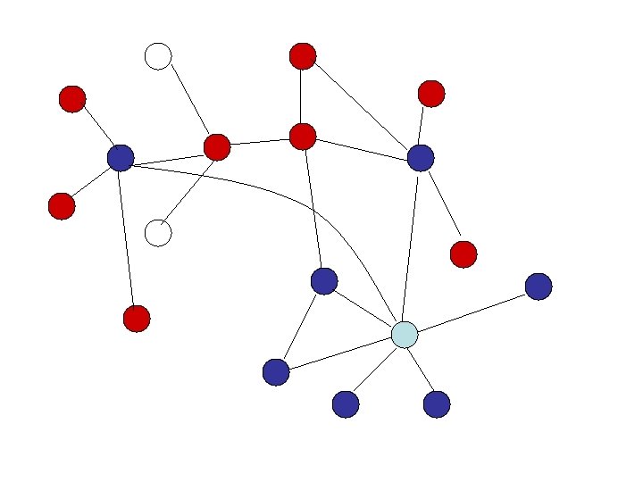
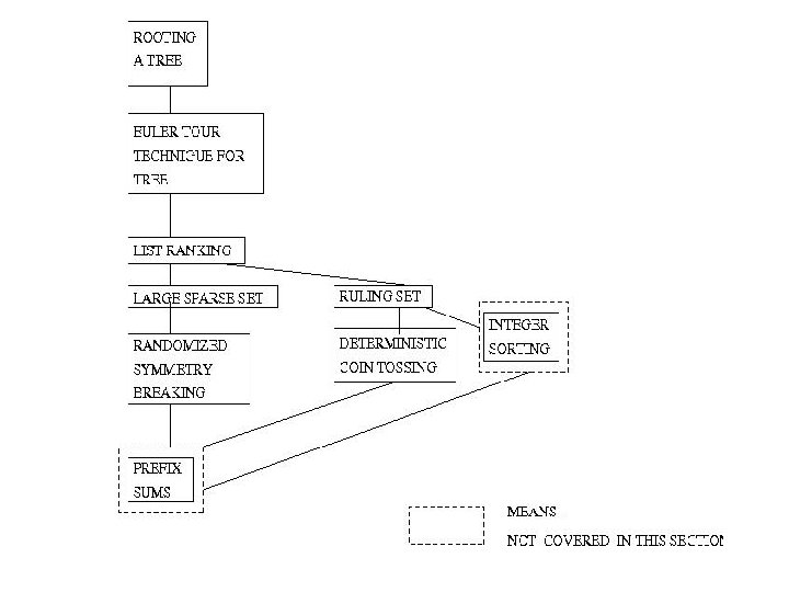
List Ranking Cluster: Euler tours; pointer jumping; randomized and deterministic symmetry breaking Tree rooting: a “toy problem” that will motivate the presentation. Input T(V, E), and some specified vertex r in V. V – vertices. E – undirected edges, contains unordered pairs of vertices. Tree rooting problem For each edge, select a direction, so that the resulting directed graph T’(V, E’) is a (directed) rooted tree whose root is vertex r; e. g. , if (u, v) is in E and vertex v is closer to the root r than vertex u then u → v is in E. Euler tour technique: constant-time optimal-work reduction of tree rooting, and other tree problems, to the list ranking problem. This section can be viewed as an extensive top-down description of an algorithm for any of these tree problems, since the list ranking algorithms that follow are also described in a top-down manner. Top-down structures of problems and techniques from the involved to the elementary have become a “trade mark” of theory of parallel algorithms, as reviewed in [Vis 91]. Such fine structures highlight the elegance of this theory and are modest, yet noteworthy, of fine structures that exist in some classical fields of Mathematics. However, they are rather unique for Combinatorics-related theories. Figure to illustrate this structure:

Tree T and its input representation The Euler-tour technique