Hash Table 1 Introduction Dictionary a dynamic set

Hash Table 1

Introduction • Dictionary: a dynamic set that supports INSERT, SEARCH, and DELETE • Hash table: an effective data structure for dictionaries – O(n) time for search in worst case – O(1) expected time for search 2

Direct-Address Tables • An Array is an example of a direct-address table – Given a key k, the corresponding is stored in T[k] • Assume no two elements have the same key – Suitable when the universe U of keys is reasonably small • U={0, 1, 2, …, m-1} T[0. . m-1] (m) • What if the no. of keys actually occurred is small • Operations of direct-address tables: all (1) time – DIRECT-ADDRESS-SEARCH(T, k): return T[k] – DIRECT-ADDRESS-INSERT(T, x): T[key[x]] x – DIRECT-ADDRESS-DELETE(T, x): T[key[x]] NIL 3

If the set contains no element with key k, T[k] = NIL 4

Alternative Illustration of Direct-Address Tables Key S 1 S 2 Key, S 1, S 2… Use separate arrays for key and satellite data if the programming language does not support objects (parallel array) If the programming language can support object-element arrays 5

Hash Tables 6

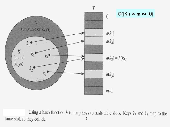
Overview • Difficulties with direct addressing – If U is large, storing a table T of size |U| may be impractical – The set K of keys actually stored may be small relative to U • When the set K of keys stored in a dictionary is much smaller than U of all possible keys, a hash table requires much less storage than a direct-address table – (|K|) storage – O(1) average time to search for an element • (1) worst case to search for an element in direct-address table 7

Hash Table • Direct addressing: an element with key k T[k] • Hash table: an element with key k T[h(k)] – h(k): hash function; usually can be computed in O(1) time • h: U {0, 1, . . , m-1} • An element with key k hashes to slot h(k) • h(k) is the hash function of key k • Instead of |U| values, we need to handle only m values – Collision may occur • Two different keys hash to the same slot (h(k 1) = h(k 2) = x) • Eliminating all collisions is impossible • But a well-designed “random”-looking hash table can minimize collisions 8

Collision Resolution by Chaining • Idea – Put all the elements that hash to the same slot in a linked list – Slot j contains a pointer to the head of the list of all stored elements that hash to j • Operations – CHAINED-HASH-INSERT(T, x): O(1) (no check for duplication) • Insert x at the head of list T[h(key[x])] – CHAINED-HASH-SEARCH(T, k): proportional to the list length • Search for an element with key k in list T[h(k)] – CHAINED-HASH-DELETE(T, x): O(1) for doubly linked list • Delete x from the list T[h(key[x])] 10

另一種方式: open addressing 11

Analysis of Hashing with Chaining for Searching • Load factor = n elements/m slots (負載因子) – Average number of elements stored in a chain • Worst case: (n) + time to compute the hash function – all n keys hash into the same slot • Average performance – How well the hash function h distributes the set of keys to be stored among the m slots, on the average – Assume simple uniform hashing • Any given element is equally likely to hash into any of the m slots, independently of where any other elements hashed to – The time required for a successful or unsuccessful search is (1+ ) • n = O(m) = n/m = O(m)/m = O(1) 12

Hash Functions 13

Overview • Interpreting keys as natural numbers N={0, 1, 2, …} – If the keys are not natural number convert For example “pt”: p=112, t=116, using radix-128 integer pt becomes 112*128+116=14452 • What makes a good hash function? – Each key is equally likely to hash to any of the m slots, independently of where any other key hashed to • Rarely knows the probability distribution • Keys may not be drawn independently – Hash by division: heuristic – Hash by multiplication: heuristic – Universal hashing: randomization to provide provably good performance 14

Hash By Division • h(k) = k mod m – m = 12 and k=100 h(k) = 4 – Must avoid certain values of m rely on characteristics of k values • m should not be a power of 2 h(k) is the lowest-order bits of k – Good values for m are primes not too close to an 2 P – For example: n=2000 character string, we don’n mind examing 3 elements in unsuccessful search allocate a hash table of size 701 is prime near 2000/3, not near any power of 2 h(k)=k mod 701 15

Hash By Multiplication • h(k) = m*(k*A mod 1) – multiply the key k by a A (0, 1) and extract the fractional part of k. A – multiply the fractional part of k. A by m and take the floor of the result • The value of m is not critical – Typically, m = 2 P (for easy implementation on computers) – (Knuth) – For example: k=123456, m=10000, a=0. 618 H(k)=floor(10000*(123456*0. 618… mod 1)) =floor(10000*(76300. 004151. . mod 1)) =floor(10000*0. 0041151…. . )=41. 16

Universal Hashing • Idea: – Choose the hash function randomly in a way that is independent of the keys that are actually going to be stored – Select the hash function at random from a carefully designed class of functions at the beginning of execution • The algorithm can behave differently on each execution, even for the same input 17

Universal Hashing (Cont. ) • Let H be a finite collection of hash functions that map a given universe U of keys into the range {0, 1, …, m-1}. • H is universal if for each pair of distinct keys k, l U, the number of hash functions h H for which k(h) = k(l) is at most |H|/m – Collision chance = 1/m • Theorem 11. 3. – Suppose that a hash function h is chosen from a universal collection of hash function and is used to hash n keys into a table T of size m, using chaining to resolve collisions. If key k is not in the table, then the expected length E[nh(k)] of the list that key k hashes to is at most . If key k is in the table, then the expected length E[nh(k)] of the list containing key k is at most 1+ 18

Designing A Universal Class of Hash Functions • Steps to design a universal class of hash functions – – Choose a prime number p, so that k [0, p-1] and p > m Zp={0, 1, …, p-1} Z*p={1, 2, …, p-1} ha, b(k) = ((ak+b) mod p) mod m, for any a Z*p and b Zp • The family of all such hash functions is – Hp, m = {ha, b: a Z*p and b Zp} – Total: p(p-1) hash functions in Hp, m 19

Other hash function(1) • Mid-square: 先將數值平方在取中 間部分位元 (39)2=(100111)2=(10111110001)2 F(39)=(11110)2=(29)10 • Digital analysis: 位數分析, 對資料 每一位數加以分析, 剔除不均勻分 布之位數, 剩下位數作為hash位址 適合static data 且位數相同 For example 20 x F(x) 1510327 5107 1857384 8574 2621439 6219 1796333 7963 1038420 0380 7142481 1421 7203326 2036 2385425 3855

Other hash function(2) • Folding(摺疊法): • (1)shift folding • (2)folding at boundaries 1214 + 3412 1511 2351 1214 3412 1511 2351 20 20 + 1214 2143 1511 1532 20 6420 8508 21

Open Addressing 22

Overview • All elements are stored in the hash table itself – Each table entry contains either an set element or NIL – Search: systematically examine table slots until the desired element is found or it is clear that the element is not in the table – No lists and no elements are stored outside the table • Load factor 1 – At most m elements can be stored in the hash table • The extra memory freed by not storing pointers provides the hash table with a larger number of slots for the same amount of memory, potentially yielding fewer collisions and faster retrieval 23

Probe • Insertion: successively examine (probe) the hash table until we find an empty slot in which to put the key – The sequence of positions probed relies on the key being inserted • Probe sequence for every key k must be a permutation of <0, 1, . . , m-1> – Extended hash function h: U * {0, 1, …, m-1} • <h(k, 0), h(k, 1), …, h(k, m-1)> • Assume uniform hashing – Each key is equally likely to have any of the m! permutations of <0, 1, …, m-1> as its probe sequence 24

INSERT and SEARCH in Open Addressing Assume keys are not deleted from the table 25

Example h’(k)=k mod 5 h(k, i)=(h’(k) + i) mod 5 For k=9 h(k, i) = <4, 0, 1, 2, 3> For k=3 h(k, i) = <3, 4, 0, 1, 2> 0 1 2 3 4 14 2 9 0 1 2 3 4 14 2 We have to mark a deleted slot, instead of letting it be NIL DELETED 9 HASH-INSERT(T, 2) HASH-DELETE(T, 9) HASH-INSERT(T, 9) HASH-SEARCH(T, 14) HASH-INSERT(T, 14) 26

DELETE in Open Addressing • Difficult !! – Cannot simply mark the deleted slot i as empty by storing NIL • Impossible to retrieve any key k during whose insertion we had probed slot i and found it occupied – Solution: mark the slot by storing in it a special value DELETED • Modify HASH-INSERT: treat a DELETED slot as a NIL slot • No modification of HASH-SEARCH is needed – Search times are no longer dependent on – Therefore, chaining is more commonly selected as a collision resolution technique when keys must be deleted 27

Linear Probing • h(k, i) = (h’(k) + i) mod m (i = 0, 1, …, m-1) – – – h’: U {0, 1, …, m-1} is called an auxiliary hash function T[h’(k)] T[h’(k)+1] … T[m-1] T[0] … T[h’(k)-1] Only m distinct probe sequences Easy to implement Problem: Primary clustering • Long runs of occupied slots tend to get longer, and the average search time increases – Secondary clustering • If two keys have the same initial probe position, then their probe sequences are the same – Example: f(x)=x, table size=19(0. . 18), data={1. 0. 5. 1. 18. 3. 8. 9. 14. 7. 5. 5. 1. 13. 12. 5} 28

Quadratic Probing • h(k, i) = (h’(k) + c 1 i+ c 2 i 2) mod m (i = 0, 1, …, m-1) h’: auxiliary hash function; c 1, c 2 0 (auxiliary constants) The values of c 1, c 2, m are constrained (See Problem 11 -3) Work much better than linear probing (alleviate primary clustering) Secondary clustering • If two keys have the same initial probe position, then their probe sequences are the same – Only m distinct probe sequences – – 29

Double Hashing: the best • h(k, i) = (h 1(k) + i*h 2(k)) mod m (i = 0, 1, …, m-1) – h 1 and h 2 are auxiliary hash functions – Depends in two ways upon the key i, since the initial probe position, the offset, or both, may vary (m 2) distinct probing sequences – The value of h 2(k) must be relative prime to the hash-table size m for the entire hash table to be searched (Exercise 11. 4 -3) • Let m = 2 P and design h 2 so that it always produces an odd number • Let m be prime and design h 2 so that it always produces a positive integer less than m – h 1(k) = k mod 701 – h 2(k) = 1 + (k mod 700) 30

Example of Double Hashing Data sequence: 69, 72, 50, 79, 98, 14 h 1(14) = 1 h 2(14) = 4 H 1(98)=98 mod 13=7 H 2(98)=1+(98 mod 11)=11 H(98, 1)=(7+11) mod 13=5 h(k, i) = (h 1(k) + i*h 2(k)) mod m h(14, 0) = 14 mod 13=1…. …. 1 st collision h(14, 1) = (1+1*(1+(14 mod 11)))mod 13=5…. 2 nd collision h(14, 2) = (1+2*(4)) mod 13=9 H 1(k)=k mod 13 H 2(k)=1+(k mod 11) 31

Analysis of Open-Address Hashing • Theorem 11. 6 – Given an open-address hash table with load factor = n/m < 1, the expected number of probes in an unsuccessful search is at most 1/(1 - ), assuming uniform hashing • If is a constant an unsuccessful search runs in O(1) time • Corollary 11. 7 – Inserting an element into an open-address hash table with load factor requires at most 1/(1 - ) probes on average, assuming uniform hashing • Theorem 11. 8 – Given an open-address hash table with load factor = n/m < 1, the expected number of probes in an successful search is at most 1/ * ln(1/(1 - )), assuming uniform hashing and that each key in the table is equally likely to be searched for • If is a constant an unsuccessful search runs in O(1) time 32

Self-Study • Proof of Theorems • Section 11. 5 Perfect Hashing – The worst-case number of memory accesses required to perform a search is O(1) 33

example • A hashed table is constructed using the division hash algorithm function with 5 buckets (a bucket at most 4 records). If the following key field values are to be placed in buckets: 3 , 5, 24, 22, 109, 10, 8, 6, 23, 28, 100, 103, 9, 39, 27, 0. – Identify the number of records in each bucket. – Which bucket overflows? no H(k)=k mod 5 • Bucket 3 overflow. 0 5 1 6 2 22 7 27 3 3 8 23 28 4 24 109 9 29 34 10 100 0 103