Hashing General idea Hash function Separate Chaining Open

Hashing • • • General idea Hash function Separate Chaining Open Addressing Rehashing

Motivation • Tree-based data structures – O(log. N) access time (Find, Insert, Delete) • Can we do better than this? – If we consider the average case rather than worst case, is there a O(1) time approach with high probability? – Hashing is such a data structure that allows for efficient insertion, deletion, and searching of keys in O(1) time on average. • Numerous applications – Symbol table of variables in Compilers – Virtual to physical memory translation in Operating Systems – String matching

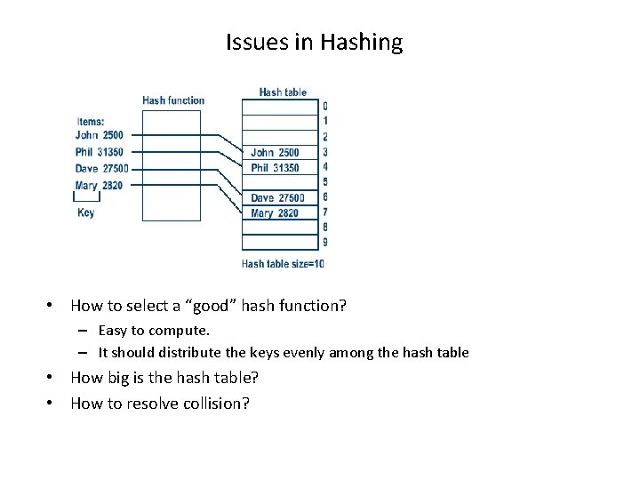
Components of Hashing • Hash table is an array of some fixed size, containing the items. – Generally a search is performed on some part of the item, called the key. – The item could consist of a string or a number (that serves as the key) and additional data members (for instance, a name that is part of a large employee structure). – The size of the table is Table. Size. • Hash function h(k) maps search key k to some location in the hash table in the range [0. . Table. Size-1]. Different keys might be mapped (or called hashed) to the same location and this is called collision.

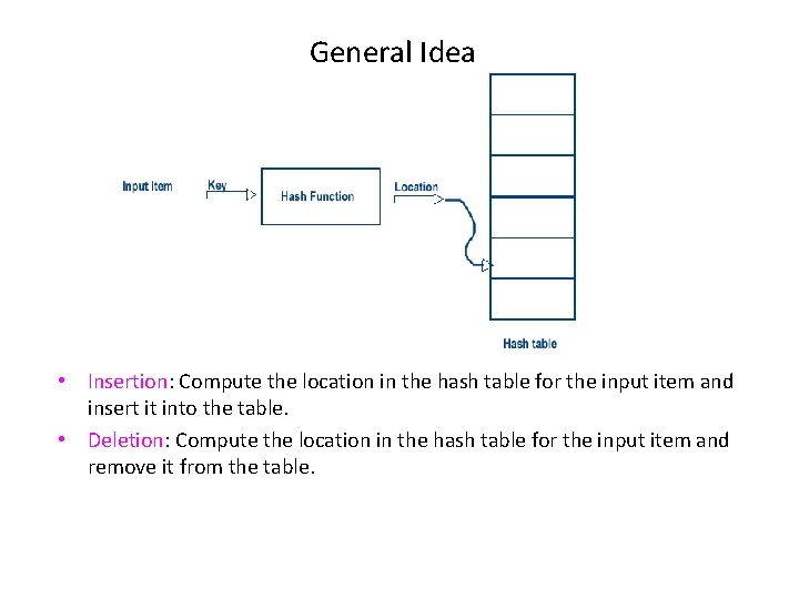
General Idea • Insertion: Compute the location in the hash table for the input item and insert it into the table. • Deletion: Compute the location in the hash table for the input item and remove it from the table.

Issues in Hashing • How to select a “good” hash function? – Easy to compute. – It should distribute the keys evenly among the hash table • How big is the hash table? • How to resolve collision?

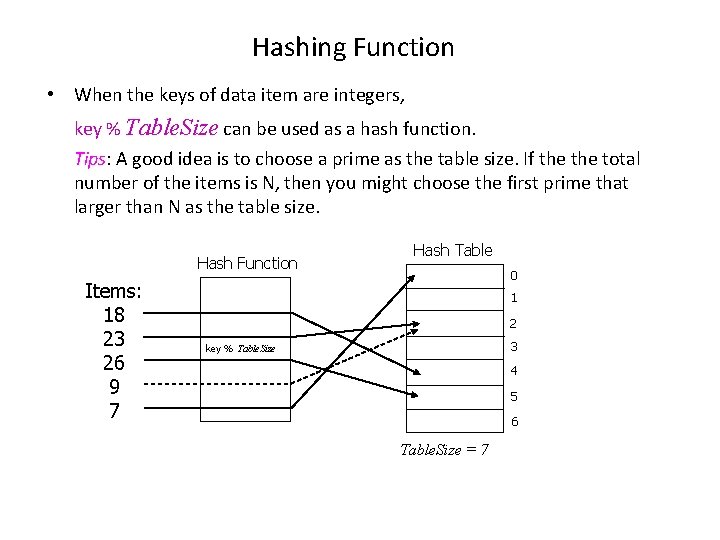
Hashing Function • When the keys of data item are integers, key % Table. Size can be used as a hash function. Tips: A good idea is to choose a prime as the table size. If the total number of the items is N, then you might choose the first prime that larger than N as the table size. Hash Function Items: 18 23 26 9 7 Hash Table 0 1 2 3 key % Table. Size 4 5 6 Table. Size = 7

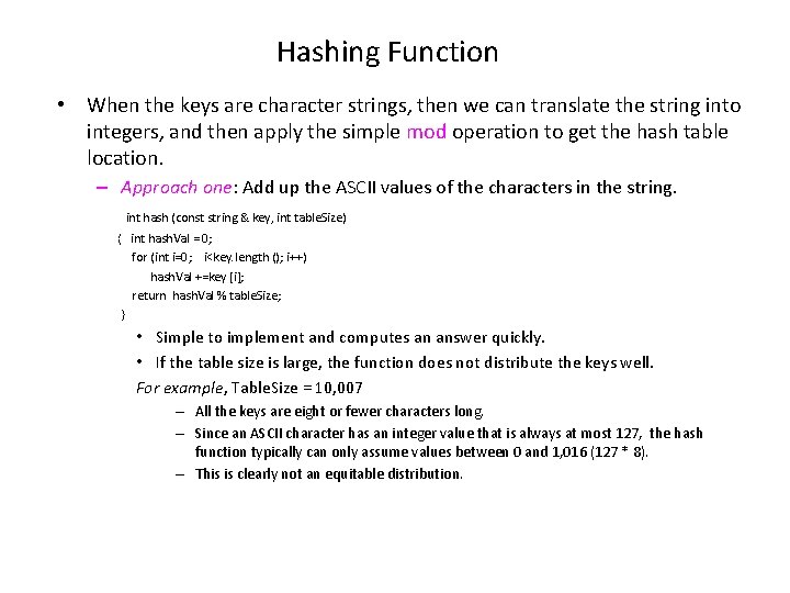
Hashing Function • When the keys are character strings, then we can translate the string into integers, and then apply the simple mod operation to get the hash table location. – Approach one: Add up the ASCII values of the characters in the string. int hash (const string & key, int table. Size) { int hash. Val = 0; for (int i=0; i<key. length (); i++) hash. Val +=key [i]; return hash. Val % table. Size; } • Simple to implement and computes an answer quickly. • If the table size is large, the function does not distribute the keys well. For example, Table. Size = 10, 007 – All the keys are eight or fewer characters long. – Since an ASCII character has an integer value that is always at most 127, the hash function typically can only assume values between 0 and 1, 016 (127 * 8). – This is clearly not an equitable distribution.

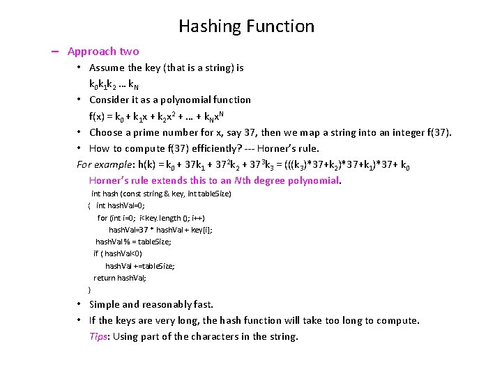
Hashing Function – Approach two • Assume the key (that is a string) is k 0 k 1 k 2 … k. N • Consider it as a polynomial function f(x) = k 0 + k 1 x + k 2 x 2 + … + k. Nx. N • Choose a prime number for x, say 37, then we map a string into an integer f(37). • How to compute f(37) efficiently? --- Horner’s rule. For example: h(k) = k 0 + 37 k 1 + 372 k 2 + 373 k 3 = (((k 3)*37+k 2)*37+k 1)*37+ k 0 Horner’s rule extends this to an Nth degree polynomial. int hash (const string & key, int table. Size) { int hash. Val=0; for (int i=0; i<key. length (); i++) hash. Val=37 * hash. Val + key[i]; hash. Val % = table. Size; if ( hash. Val<0) hash. Val +=table. Size; return hash. Val; } • Simple and reasonably fast. • If the keys are very long, the hash function will take too long to compute. Tips: Using part of the characters in the string.

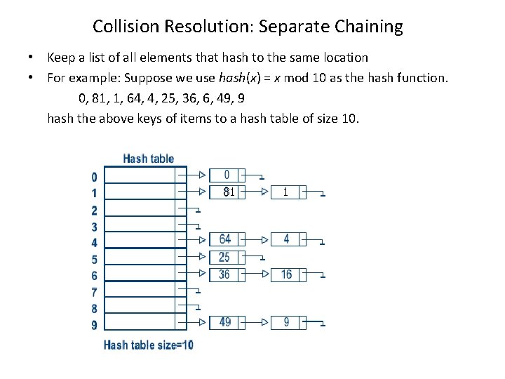
Collision Resolution: Separate Chaining • Keep a list of all elements that hash to the same location • For example: Suppose we use hash(x) = x mod 10 as the hash function. 0, 81, 1, 64, 4, 25, 36, 6, 49, 9 hash the above keys of items to a hash table of size 10. 81 1

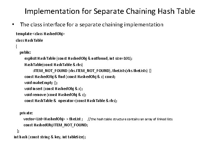
Implementation for Separate Chaining Hash Table • The class interface for a separate chaining implementation template <class Hashed. Obj> class Hash. Table { public: explicit Hash. Table (const Hashed. Obj & notfound, int size=101); Hash. Table(const Hash. Table & rhs) : ITEM_NOT_FOUND (rhs. ITEM_NOT_FOUND), the. Lists(rhs. the. Lists) {} const Hashed. Obj & find (const Hashed. Obj & x) const; void make. Empty (); void insert (const Hashed. Obj & x); void remove (const Hashed. Obj & x); const Hash. Table & operator=(const Hash. Table & rhs); private: vector<List<Hashed. Obj> > the. List ; //the hash table structure contains an array of linked lists. const Hashed. Obj ITEM_NOT_FOUND; }; int hash (const string & key, int table. Size);

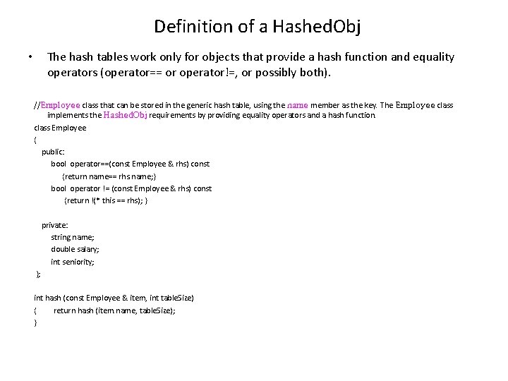
Definition of a Hashed. Obj • The hash tables work only for objects that provide a hash function and equality operators (operator== or operator!=, or possibly both). //Employee class that can be stored in the generic hash table, using the name member as the key. The Employee class implements the Hashed. Obj requirements by providing equality operators and a hash function. class Employee { public: bool operator==(const Employee & rhs) const {return name== rhs. name; } bool operator != (const Employee & rhs) const {return !(* this == rhs); } private: string name; double salary; int seniority; }; int hash (const Employee & item, int table. Size) { return hash (item. name, table. Size); }

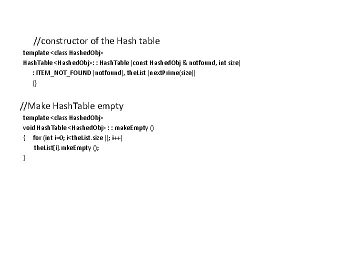
//constructor of the Hash table template <class Hashed. Obj> Hash. Table <Hashed. Obj>: : Hash. Table (const Hashed. Obj & notfound, int size) : ITEM_NOT_FOUND (notfound), the. List (next. Prime(size)) {} //Make Hash. Table empty template <class Hashed. Obj> void Hash. Table <Hashed. Obj> : : make. Empty () { for (int i=0; i<the. List. size (); i++) the. List[i]. mke. Empty (); }

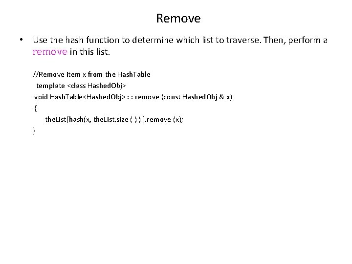
Remove • Use the hash function to determine which list to traverse. Then, perform a remove in this list. //Remove item x from the Hash. Table template <class Hashed. Obj> void Hash. Table<Hashed. Obj> : : remove (const Hashed. Obj & x) { the. List[hash(x, the. List. size ( ) ) ]. remove (x); }

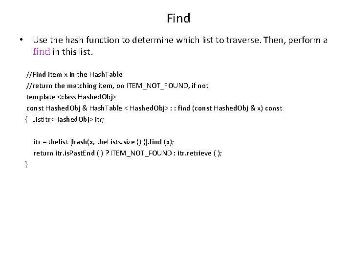
Find • Use the hash function to determine which list to traverse. Then, perform a find in this list. //Find item x in the Hash. Table //return the matching item, on ITEM_NOT_FOUND, if not template <class Hashed. Obj> const Hashed. Obj & Hash. Table < Hashed. Obj> : : find (const Hashed. Obj & x) const { List. Itr<Hashed. Obj> itr; itr = thelist [hash(x, the. Lists. size () )]. find (x); return itr. is. Past. End ( ) ? ITEM_NOT_FOUND : itr. retrieve ( ); }

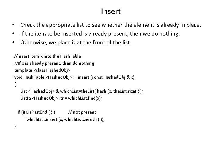
Insert • Check the appropriate list to see whether the element is already in place. • If the item to be inserted is already present, then we do nothing. • Otherwise, we place it at the front of the list. //Insert item x into the Hash. Table //If x is already present, then do nothing template <class Hashed. Obj> void Hash. Table <Hashed. Obj> : : insert (const Hashed. Obj & x) { List <Hashed. Obj> & which. List=the. List[ hash (x, the. List. size( ) ]; List. Itr<Hashed. Obj> itr = which. List. find(x); if (itr. is. Past. End ( ) ) // not present which. List. insert (x, which. List. zeroth ( )); }

Disadvantage of Separate Chaining Hashing • This implementation tends to slow the algorithm down a bit because of the time required to allocate new cells, and also essentially requires the implementation of a second data structure.

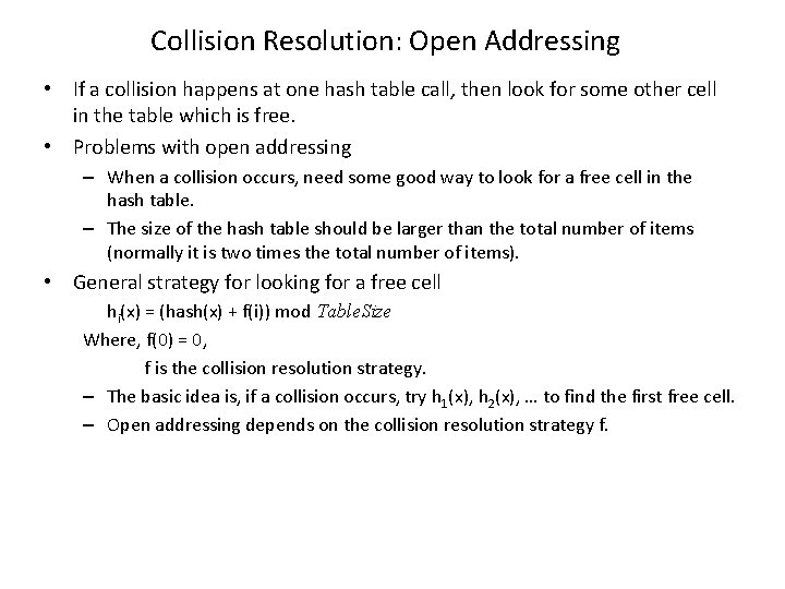
Collision Resolution: Open Addressing • If a collision happens at one hash table call, then look for some other cell in the table which is free. • Problems with open addressing – When a collision occurs, need some good way to look for a free cell in the hash table. – The size of the hash table should be larger than the total number of items (normally it is two times the total number of items). • General strategy for looking for a free cell hi(x) = (hash(x) + f(i)) mod Table. Size Where, f(0) = 0, f is the collision resolution strategy. – The basic idea is, if a collision occurs, try h 1(x), h 2(x), … to find the first free cell. – Open addressing depends on the collision resolution strategy f.

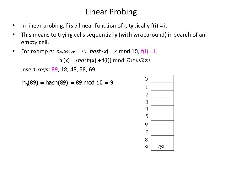
Linear Probing • In linear probing, f is a linear function of i, typically f(i) = i. • This means to trying cells sequentially (with wraparound) in search of an empty cell. • For example: Table. Size = 10, hash(x) = x mod 10, f(i) = i, hi(x) = (hash(x) + f(i)) mod Table. Size Insert keys: 89, 18, 49, 58, 69 h 0(89) = hash(89) = 89 mod 10 = 9 0 1 2 3 4 5 6 7 8 9 89

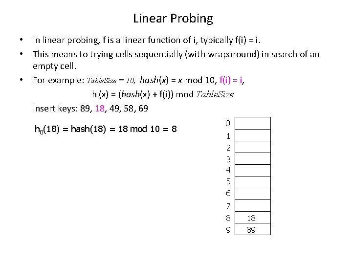
Linear Probing • In linear probing, f is a linear function of i, typically f(i) = i. • This means to trying cells sequentially (with wraparound) in search of an empty cell. • For example: Table. Size = 10, hash(x) = x mod 10, f(i) = i, hi(x) = (hash(x) + f(i)) mod Table. Size Insert keys: 89, 18, 49, 58, 69 h 0(18) = hash(18) = 18 mod 10 = 8 0 1 2 3 4 5 6 7 8 9 18 89

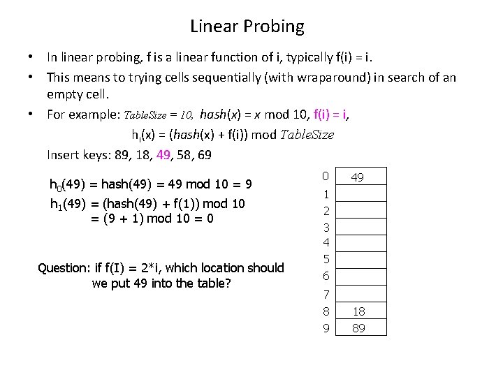
Linear Probing • In linear probing, f is a linear function of i, typically f(i) = i. • This means to trying cells sequentially (with wraparound) in search of an empty cell. • For example: Table. Size = 10, hash(x) = x mod 10, f(i) = i, hi(x) = (hash(x) + f(i)) mod Table. Size Insert keys: 89, 18, 49, 58, 69 h 0(49) = hash(49) = 49 mod 10 = 9 h 1(49) = (hash(49) + f(1)) mod 10 = (9 + 1) mod 10 = 0 Question: if f(I) = 2*i, which location should we put 49 into the table? 0 49 1 2 3 4 5 6 7 8 9 18 89

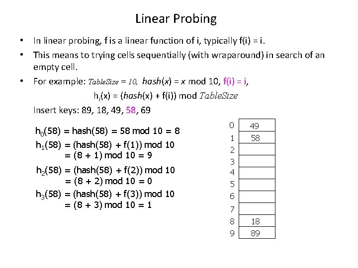
Linear Probing • In linear probing, f is a linear function of i, typically f(i) = i. • This means to trying cells sequentially (with wraparound) in search of an empty cell. • For example: Table. Size = 10, hash(x) = x mod 10, f(i) = i, hi(x) = (hash(x) + f(i)) mod Table. Size Insert keys: 89, 18, 49, 58, 69 h 0(58) = hash(58) = 58 mod 10 = 8 h 1(58) = (hash(58) + f(1)) mod 10 = (8 + 1) mod 10 = 9 h 2(58) = (hash(58) + f(2)) mod 10 = (8 + 2) mod 10 = 0 h 3(58) = (hash(58) + f(3)) mod 10 = (8 + 3) mod 10 = 1 0 1 2 3 4 5 6 7 8 9 49 58 18 89

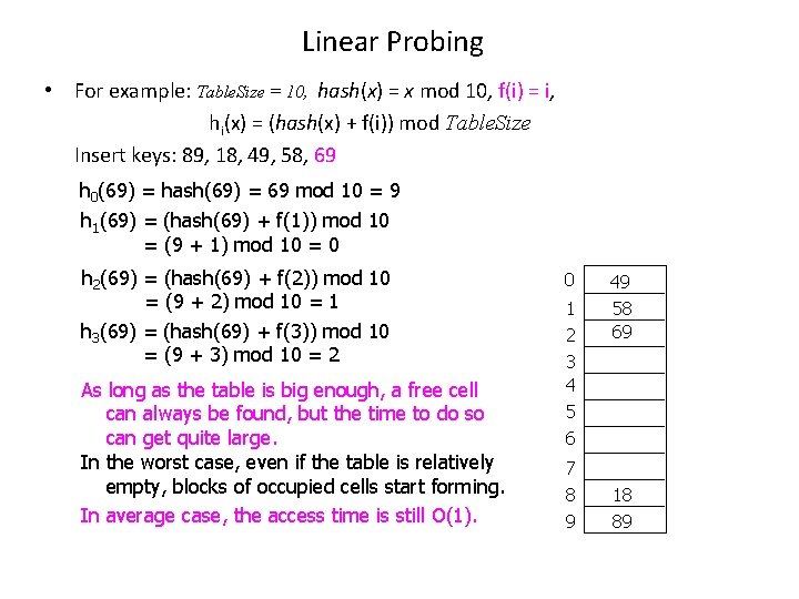
Linear Probing • For example: Table. Size = 10, hash(x) = x mod 10, f(i) = i, hi(x) = (hash(x) + f(i)) mod Table. Size Insert keys: 89, 18, 49, 58, 69 h 0(69) = hash(69) = 69 mod 10 = 9 h 1(69) = (hash(69) + f(1)) mod 10 = (9 + 1) mod 10 = 0 h 2(69) = (hash(69) + f(2)) mod 10 = (9 + 2) mod 10 = 1 h 3(69) = (hash(69) + f(3)) mod 10 = (9 + 3) mod 10 = 2 As long as the table is big enough, a free cell can always be found, but the time to do so can get quite large. In the worst case, even if the table is relatively empty, blocks of occupied cells start forming. In average case, the access time is still O(1). 0 1 2 3 4 5 6 7 8 9 49 58 69 18 89

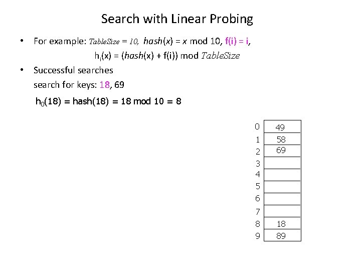
Search with Linear Probing • For example: Table. Size = 10, hash(x) = x mod 10, f(i) = i, hi(x) = (hash(x) + f(i)) mod Table. Size • Successful searches search for keys: 18, 69 h 0(18) = hash(18) = 18 mod 10 = 8 0 1 2 3 4 5 6 7 8 9 49 58 69 18 89

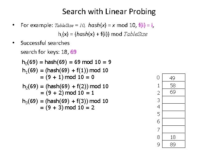
Search with Linear Probing • For example: Table. Size = 10, hash(x) = x mod 10, f(i) = i, hi(x) = (hash(x) + f(i)) mod Table. Size • Successful searches search for keys: 18, 69 h 0(69) = hash(69) = 69 mod 10 = 9 h 1(69) = (hash(69) + f(1)) mod 10 = (9 + 1) mod 10 = 0 h 2(69) = (hash(69) + f(2)) mod 10 = (9 + 2) mod 10 = 1 h 3(69) = (hash(69) + f(3)) mod 10 = (9 + 3) mod 10 = 2 0 1 2 3 4 5 6 7 8 9 49 58 69 18 89

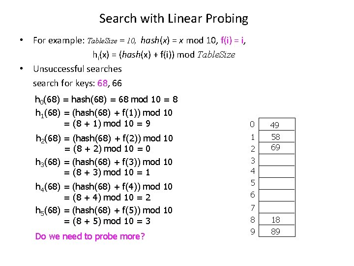
Search with Linear Probing • For example: Table. Size = 10, hash(x) = x mod 10, f(i) = i, hi(x) = (hash(x) + f(i)) mod Table. Size • Unsuccessful searches search for keys: 68, 66 h 0(68) = hash(68) = 68 mod 10 = 8 h 1(68) = (hash(68) + f(1)) mod 10 = (8 + 1) mod 10 = 9 h 2(68) = (hash(68) + f(2)) mod 10 = (8 + 2) mod 10 = 0 h 3(68) = (hash(68) + f(3)) mod 10 = (8 + 3) mod 10 = 1 h 4(68) = (hash(68) + f(4)) mod 10 = (8 + 4) mod 10 = 2 h 5(68) = (hash(68) + f(5)) mod 10 = (8 + 5) mod 10 = 3 Do we need to probe more? 0 1 2 3 4 5 6 7 8 9 49 58 69 18 89

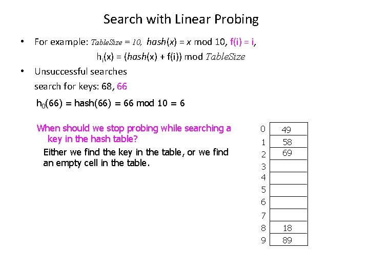
Search with Linear Probing • For example: Table. Size = 10, hash(x) = x mod 10, f(i) = i, hi(x) = (hash(x) + f(i)) mod Table. Size • Unsuccessful searches search for keys: 68, 66 h 0(66) = hash(66) = 66 mod 10 = 6 When should we stop probing while searching a key in the hash table? Either we find the key in the table, or we find an empty cell in the table. 0 1 2 3 4 5 6 7 8 9 49 58 69 18 89

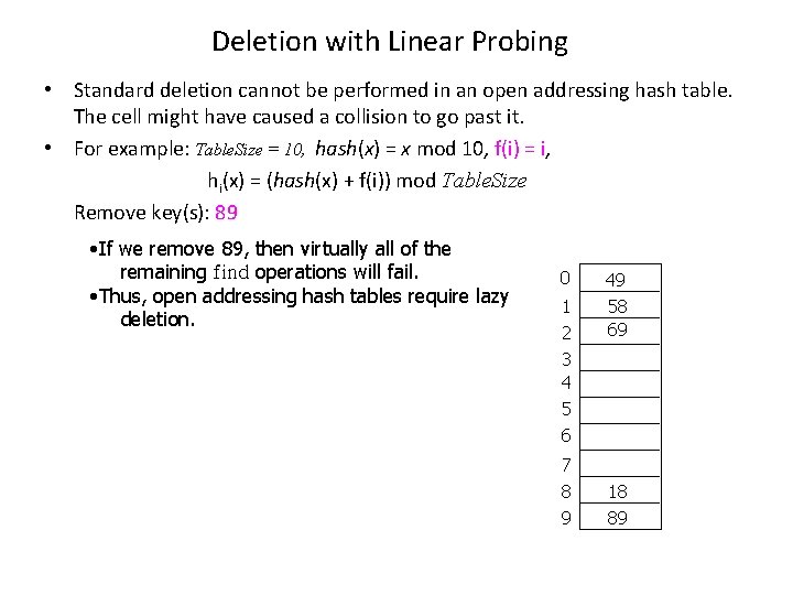
Deletion with Linear Probing • Standard deletion cannot be performed in an open addressing hash table. The cell might have caused a collision to go past it. • For example: Table. Size = 10, hash(x) = x mod 10, f(i) = i, hi(x) = (hash(x) + f(i)) mod Table. Size Remove key(s): 89 • If we remove 89, then virtually all of the remaining find operations will fail. • Thus, open addressing hash tables require lazy deletion. 0 1 2 3 4 5 6 7 8 9 49 58 69 18 89

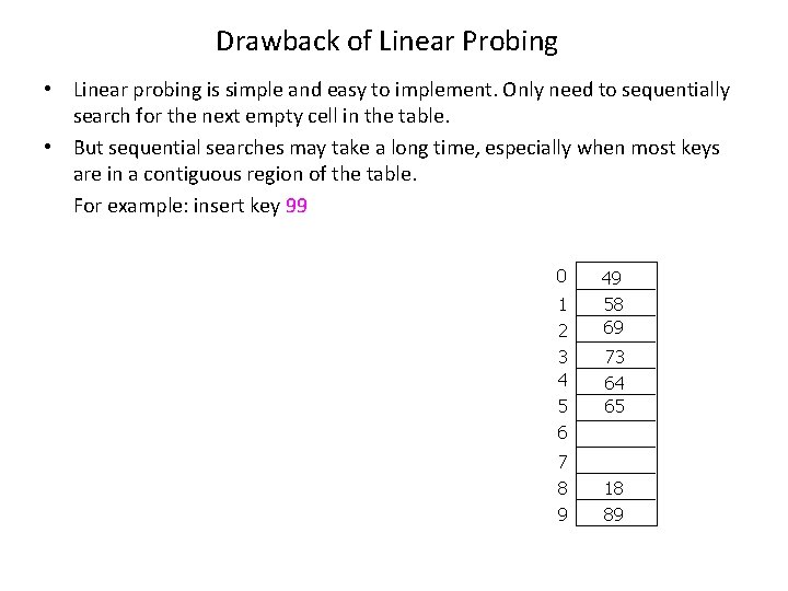
Drawback of Linear Probing • Linear probing is simple and easy to implement. Only need to sequentially search for the next empty cell in the table. • But sequential searches may take a long time, especially when most keys are in a contiguous region of the table. For example: insert key 99 0 1 2 3 4 5 6 7 8 9 49 58 69 73 64 65 18 89

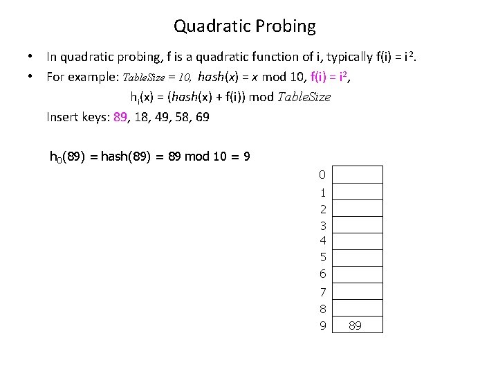
Quadratic Probing • In quadratic probing, f is a quadratic function of i, typically f(i) = i 2. • For example: Table. Size = 10, hash(x) = x mod 10, f(i) = i 2, hi(x) = (hash(x) + f(i)) mod Table. Size Insert keys: 89, 18, 49, 58, 69 h 0(89) = hash(89) = 89 mod 10 = 9 0 1 2 3 4 5 6 7 8 9 89

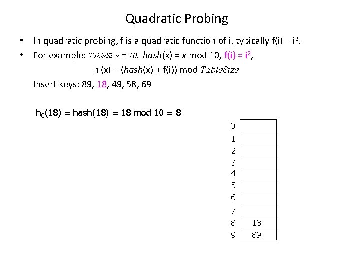
Quadratic Probing • In quadratic probing, f is a quadratic function of i, typically f(i) = i 2. • For example: Table. Size = 10, hash(x) = x mod 10, f(i) = i 2, hi(x) = (hash(x) + f(i)) mod Table. Size Insert keys: 89, 18, 49, 58, 69 h 0(18) = hash(18) = 18 mod 10 = 8 0 1 2 3 4 5 6 7 8 9 18 89

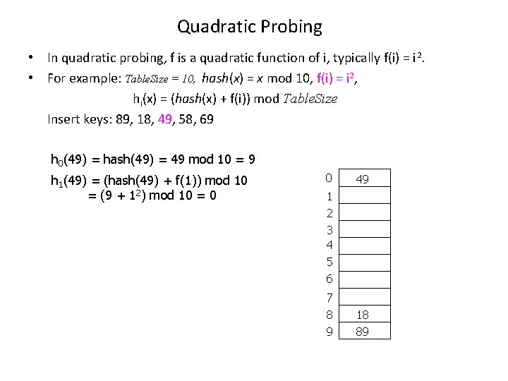
Quadratic Probing • In quadratic probing, f is a quadratic function of i, typically f(i) = i 2. • For example: Table. Size = 10, hash(x) = x mod 10, f(i) = i 2, hi(x) = (hash(x) + f(i)) mod Table. Size Insert keys: 89, 18, 49, 58, 69 h 0(49) = hash(49) = 49 mod 10 = 9 h 1(49) = (hash(49) + f(1)) mod 10 = (9 + 12) mod 10 = 0 0 49 1 2 3 4 5 6 7 8 9 18 89

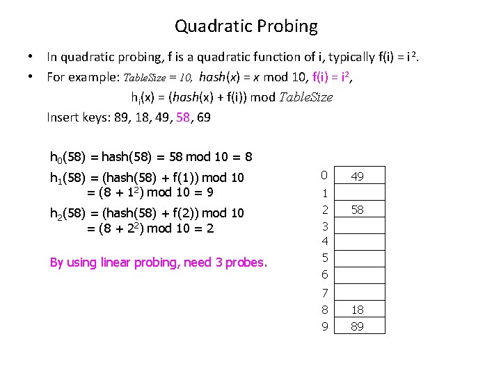
Quadratic Probing • In quadratic probing, f is a quadratic function of i, typically f(i) = i 2. • For example: Table. Size = 10, hash(x) = x mod 10, f(i) = i 2, hi(x) = (hash(x) + f(i)) mod Table. Size Insert keys: 89, 18, 49, 58, 69 h 0(58) = hash(58) = 58 mod 10 = 8 h 1(58) = (hash(58) + f(1)) mod 10 = (8 + 12) mod 10 = 9 h 2(58) = (hash(58) + f(2)) mod 10 = (8 + 22) mod 10 = 2 By using linear probing, need 3 probes. 0 1 2 3 4 5 6 7 8 9 49 58 18 89

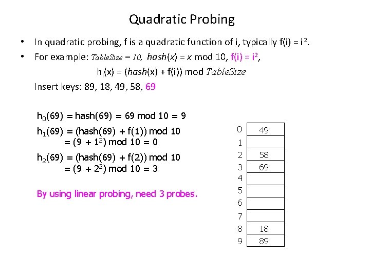
Quadratic Probing • In quadratic probing, f is a quadratic function of i, typically f(i) = i 2. • For example: Table. Size = 10, hash(x) = x mod 10, f(i) = i 2, hi(x) = (hash(x) + f(i)) mod Table. Size Insert keys: 89, 18, 49, 58, 69 h 0(69) = hash(69) = 69 mod 10 = 9 h 1(69) = (hash(69) + f(1)) mod 10 = (9 + 12) mod 10 = 0 h 2(69) = (hash(69) + f(2)) mod 10 = (9 + 22) mod 10 = 3 By using linear probing, need 3 probes. 0 1 2 3 4 5 6 7 8 9 49 58 69 18 89

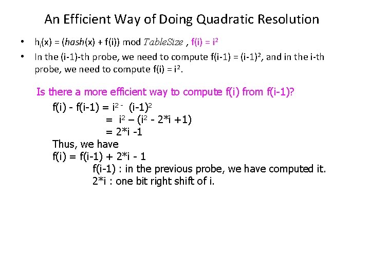
An Efficient Way of Doing Quadratic Resolution • hi(x) = (hash(x) + f(i)) mod Table. Size , f(i) = i 2 • In the (i-1)-th probe, we need to compute f(i-1) = (i-1)2, and in the i-th probe, we need to compute f(i) = i 2. Is there a more efficient way to compute f(i) from f(i-1)? f(i) - f(i-1) = i 2 - (i-1)2 = i 2 – (i 2 - 2*i +1) = 2*i -1 Thus, we have f(i) = f(i-1) + 2*i - 1 f(i-1) : in the previous probe, we have computed it. 2*i : one bit right shift of i.

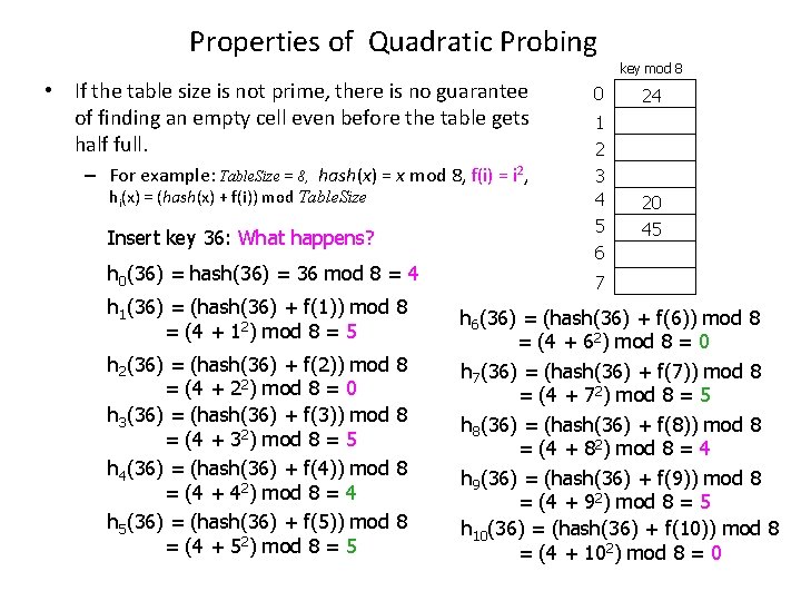
Properties of Quadratic Probing key mod 8 • If the table size is not prime, there is no guarantee of finding an empty cell even before the table gets half full. 0 – For example: Table. Size = 8, hash(x) = x mod 8, f(i) = i 2, 3 4 5 6 hi(x) = (hash(x) + f(i)) mod Table. Size Insert key 36: What happens? h 0(36) = hash(36) = 36 mod 8 = 4 h 1(36) = (hash(36) + f(1)) mod 8 = (4 + 12) mod 8 = 5 h 2(36) = (hash(36) + f(2)) mod = (4 + 22) mod 8 = 0 h 3(36) = (hash(36) + f(3)) mod = (4 + 32) mod 8 = 5 h 4(36) = (hash(36) + f(4)) mod = (4 + 42) mod 8 = 4 h 5(36) = (hash(36) + f(5)) mod = (4 + 52) mod 8 = 5 8 8 24 1 2 20 45 7 h 6(36) = (hash(36) + f(6)) mod 8 = (4 + 62) mod 8 = 0 h 7(36) = (hash(36) + f(7)) mod 8 = (4 + 72) mod 8 = 5 h 8(36) = (hash(36) + f(8)) mod 8 = (4 + 82) mod 8 = 4 h 9(36) = (hash(36) + f(9)) mod 8 = (4 + 92) mod 8 = 5 h 10(36) = (hash(36) + f(10)) mod 8 = (4 + 102) mod 8 = 0

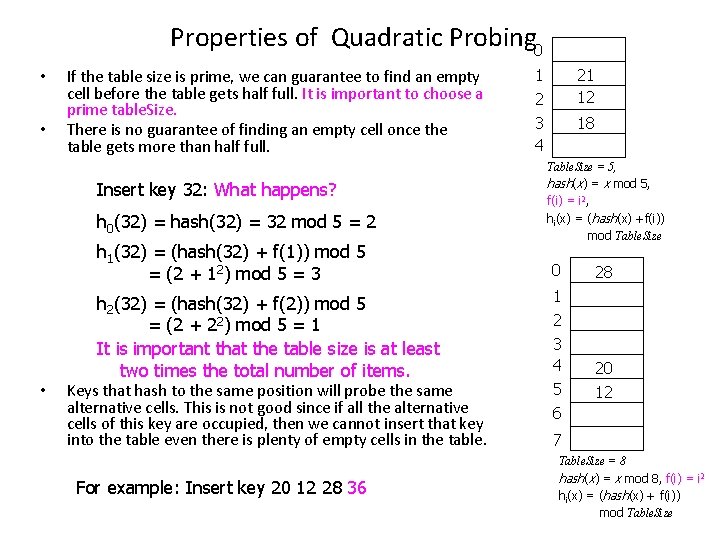
Properties of Quadratic Probing 0 • • If the table size is prime, we can guarantee to find an empty cell before the table gets half full. It is important to choose a prime table. Size. There is no guarantee of finding an empty cell once the table gets more than half full. Insert key 32: What happens? h 0(32) = hash(32) = 32 mod 5 = 2 h 1(32) = (hash(32) + f(1)) mod 5 = (2 + 12) mod 5 = 3 h 2(32) = (hash(32) + f(2)) mod 5 = (2 + 22) mod 5 = 1 It is important that the table size is at least two times the total number of items. • Keys that hash to the same position will probe the same alternative cells. This is not good since if all the alternative cells of this key are occupied, then we cannot insert that key into the table even there is plenty of empty cells in the table. For example: Insert key 20 12 28 36 1 2 21 12 3 4 18 Table. Size = 5, hash(x) = x mod 5, f(i) = i 2, hi(x) = (hash(x) +f(i)) mod Table. Size 0 28 1 2 3 4 5 20 12 6 7 Table. Size = 8 hash(x) = x mod 8, f(i) = i 2 hi(x) = (hash(x) + f(i)) mod Table. Size

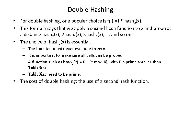
Double Hashing • For double hashing, one popular choice is f(i) = i * hash 2(x). • This formula says that we apply a second hash function to x and probe at a distance hash 2(x), 2 hash 2(x), 3 hash 2(x), …, and so on. • The choice of hash 2(x) is essential. – The function must never evaluate to zero. – It is important to make sure all cells can be probed. – A function such as hash 2(x) = R – (x mod R), with R a prime smaller than Table. Size. – Table. Size need to be prime. • The cost of double hashing: the use of a second hash function.

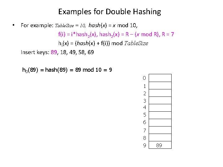
Examples for Double Hashing • For example: Table. Size = 10, hash(x) = x mod 10, f(i) = i*hash 2(x), hash 2(x) = R – (x mod R), R = 7 hi(x) = (hash(x) + f(i)) mod Table. Size Insert keys: 89, 18, 49, 58, 69 h 0(89) = hash(89) = 89 mod 10 = 9 0 1 2 3 4 5 6 7 8 9 89

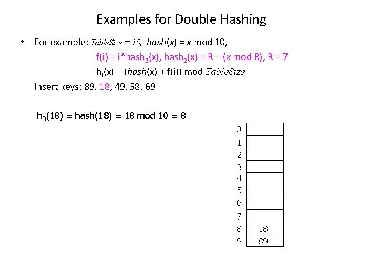
Examples for Double Hashing • For example: Table. Size = 10, hash(x) = x mod 10, f(i) = i*hash 2(x), hash 2(x) = R – (x mod R), R = 7 hi(x) = (hash(x) + f(i)) mod Table. Size Insert keys: 89, 18, 49, 58, 69 h 0(18) = hash(18) = 18 mod 10 = 8 0 1 2 3 4 5 6 7 8 9 18 89

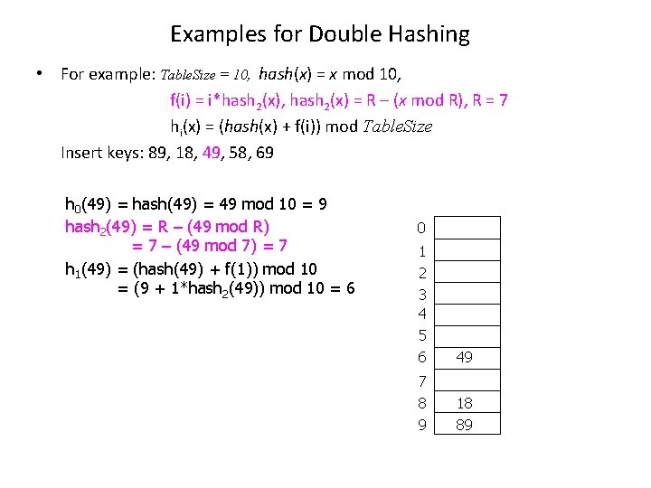
Examples for Double Hashing • For example: Table. Size = 10, hash(x) = x mod 10, f(i) = i*hash 2(x), hash 2(x) = R – (x mod R), R = 7 hi(x) = (hash(x) + f(i)) mod Table. Size Insert keys: 89, 18, 49, 58, 69 h 0(49) = hash(49) = 49 mod 10 = 9 hash 2(49) = R – (49 mod R) = 7 – (49 mod 7) = 7 h 1(49) = (hash(49) + f(1)) mod 10 = (9 + 1*hash 2(49)) mod 10 = 6 0 1 2 3 4 5 6 49 7 8 9 18 89

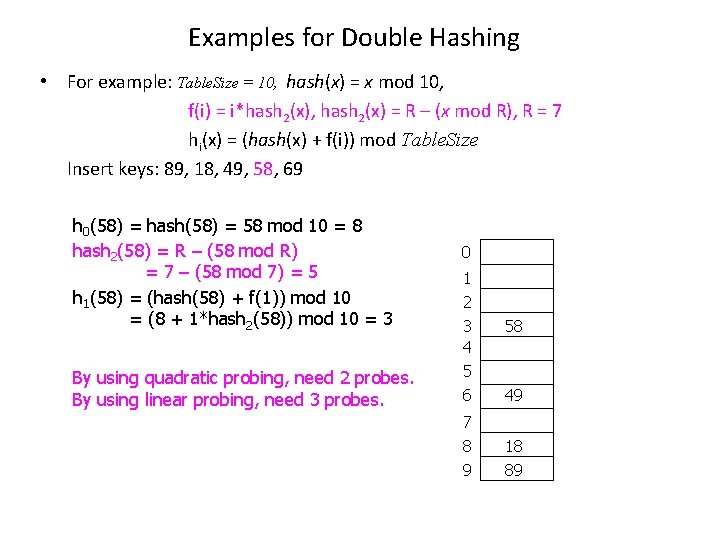
Examples for Double Hashing • For example: Table. Size = 10, hash(x) = x mod 10, f(i) = i*hash 2(x), hash 2(x) = R – (x mod R), R = 7 hi(x) = (hash(x) + f(i)) mod Table. Size Insert keys: 89, 18, 49, 58, 69 h 0(58) = hash(58) = 58 mod 10 = 8 hash 2(58) = R – (58 mod R) = 7 – (58 mod 7) = 5 h 1(58) = (hash(58) + f(1)) mod 10 = (8 + 1*hash 2(58)) mod 10 = 3 By using quadratic probing, need 2 probes. By using linear probing, need 3 probes. 0 1 2 3 4 5 6 7 8 9 58 49 18 89

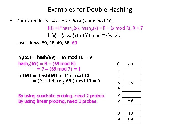
Examples for Double Hashing • For example: Table. Size = 10, hash(x) = x mod 10, f(i) = i*hash 2(x), hash 2(x) = R – (x mod R), R = 7 hi(x) = (hash(x) + f(i)) mod Table. Size Insert keys: 89, 18, 49, 58, 69 h 0(69) = hash(69) = 69 mod 10 = 9 hash 2(69) = R – (69 mod R) = 7 – (69 mod 7) = 1 h 1(69) = (hash(69) + f(1)) mod 10 = (9 + 1*hash 2(69)) mod 10 = 0 By using quadratic probing, need 2 probes. By using linear probing, need 3 probes. 0 1 2 3 4 5 6 7 8 9 69 58 49 18 89

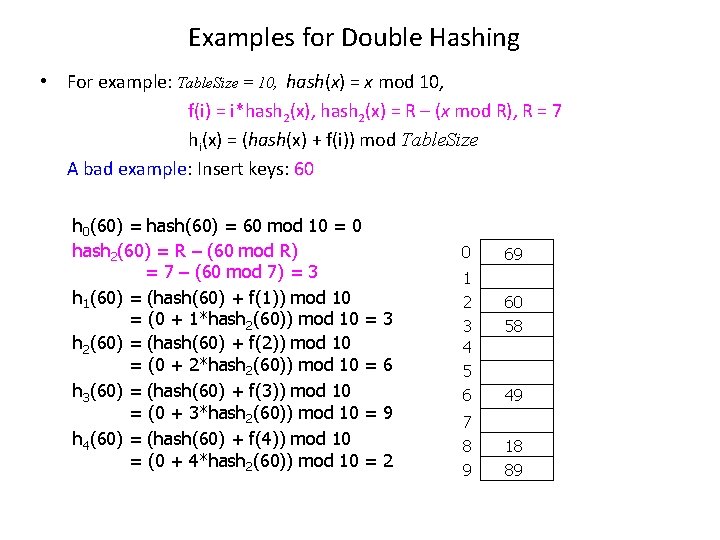
Examples for Double Hashing • For example: Table. Size = 10, hash(x) = x mod 10, f(i) = i*hash 2(x), hash 2(x) = R – (x mod R), R = 7 hi(x) = (hash(x) + f(i)) mod Table. Size A bad example: Insert keys: 60 h 0(60) = hash(60) = 60 mod 10 = 0 hash 2(60) = R – (60 mod R) = 7 – (60 mod 7) = 3 h 1(60) = (hash(60) + f(1)) mod 10 = (0 + 1*hash 2(60)) mod 10 = h 2(60) = (hash(60) + f(2)) mod 10 = (0 + 2*hash 2(60)) mod 10 = h 3(60) = (hash(60) + f(3)) mod 10 = (0 + 3*hash 2(60)) mod 10 = h 4(60) = (hash(60) + f(4)) mod 10 = (0 + 4*hash 2(60)) mod 10 = 0 3 6 9 2 1 2 3 4 5 6 7 8 9 69 60 58 49 18 89

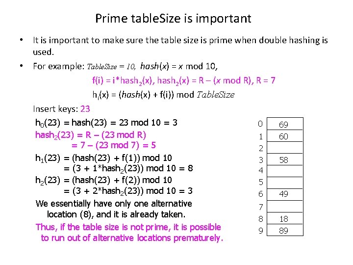
Prime table. Size is important • It is important to make sure the table size is prime when double hashing is used. • For example: Table. Size = 10, hash(x) = x mod 10, f(i) = i*hash 2(x), hash 2(x) = R – (x mod R), R = 7 hi(x) = (hash(x) + f(i)) mod Table. Size Insert keys: 23 h 0(23) = hash(23) = 23 mod 10 = 3 hash 2(23) = R – (23 mod R) = 7 – (23 mod 7) = 5 h 1(23) = (hash(23) + f(1)) mod 10 = (3 + 1*hash 2(23)) mod 10 = 8 h 2(23) = (hash(23) + f(2)) mod 10 = (3 + 2*hash 2(23)) mod 10 = 3 We essentially have only one alternative location (8), and it is already taken. Thus, if the table size is not prime, it is possible to run out of alternative locations prematurely. 0 1 2 3 4 5 6 7 8 9 69 60 58 49 18 89

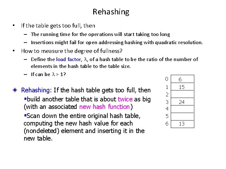
Rehashing • If the table gets too full, then – The running time for the operations will start taking too long – Insertions might fail for open addressing hashing with quadratic resolution. • How to measure the degree of fullness? – Define the load factor, , of a hash table to be the ratio of the number of elements in the hash table to the table size. – If can be > 1? 0 Rehashing: If the hash table gets too full, then §build another table that is about twice as big (with an associated new hash function) §Scan down the entire original hash table, computing the new hash value for each (nondeleted) element and inserting it in the new table. 1 2 3 4 5 6 6 15 24 13

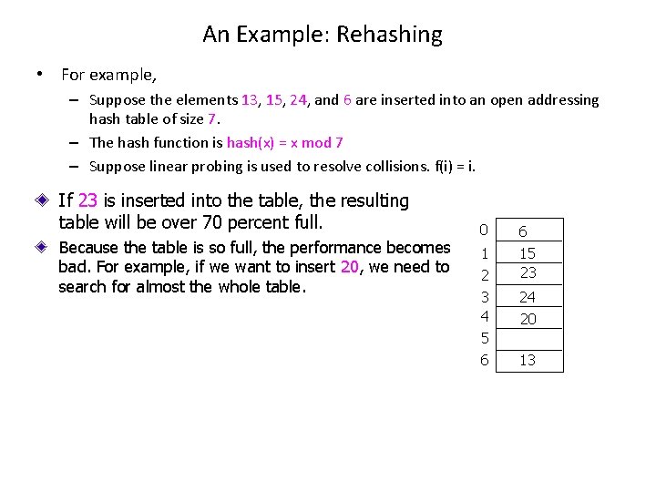
An Example: Rehashing • For example, – Suppose the elements 13, 15, 24, and 6 are inserted into an open addressing hash table of size 7. – The hash function is hash(x) = x mod 7 – Suppose linear probing is used to resolve collisions. f(i) = i. If 23 is inserted into the table, the resulting table will be over 70 percent full. Because the table is so full, the performance becomes bad. For example, if we want to insert 20, we need to search for almost the whole table. 0 1 2 3 4 5 6 6 15 23 24 20 13

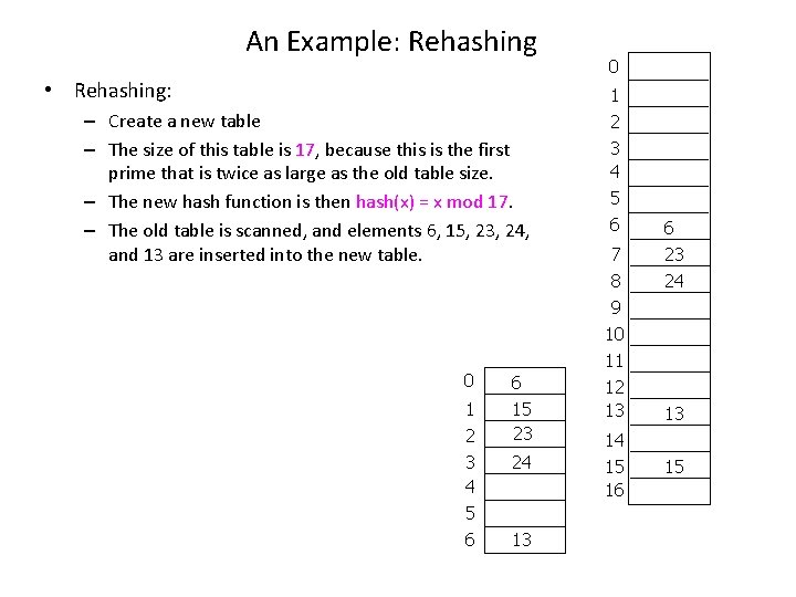
An Example: Rehashing • Rehashing: – Create a new table – The size of this table is 17, because this is the first prime that is twice as large as the old table size. – The new hash function is then hash(x) = x mod 17. – The old table is scanned, and elements 6, 15, 23, 24, and 13 are inserted into the new table. 0 1 2 3 4 5 6 6 15 23 24 13 0 1 2 3 4 5 6 7 8 9 10 11 12 13 6 23 24 13 14 15 16 15

Running Time of Rehashing • Rehashing is obviously a very expensive operation; the running time is O(N). – There are N elements to rehash and the table size is roughly 2 N. • However, it is actually not all that bad, because it happens very infrequently. • In particular, there must have been N/2 insertions prior to the last rehash, so it essentially adds a constant cost to each insertion.

When to do Rehashing? • Rehashing can be implemented in several ways with quadratic probing. – One alternative is to rehash as soon as the table is half full. – The other extreme is to rehash only when an insertion fails. – A third, middle-of-the-road strategy is to rehash when the table reaches a certain load factor. • Since performance does degrade as the load factor increases, the third strategy, implemented with a good cutoff, could be best. • Rehashing frees the programmer from worrying about the table size and is important because hash tables cannot be made arbitrarily large in complex programs.

Summary • Hash tables can be used to implement the insert and find operations in constant average time. • For separate chaining hashing, the load factor should be close to 1, although performance does not significantly degrade unless the load factor becomes very large. • For open addressing hashing, the load factor should not exceed 0. 5, unless this is completely unavoidable. – If linear probing is used, performance degenerates rapidly as the load factor approaches 1. • Rehashing can be implemented to allow the table to grow (and shrink), thus maintaining a reasonable load factor. • Disadvantage of hashing: do not support routines that require order. – Using a hash table, it is not possible to find the minimum (maximum) element efficiently. – It is not possible to search efficiently for a string unless the exact string is known. – It is not supported to quickly find all items in a certain range.