Group Analysis iwi Parker Jones SPM Course London

Group Analysis ‘Ōiwi Parker Jones SPM Course, London May 2015

Overview Variation may come from multiple sources Some common to all data, e. g. measurement noise Some common to subsets, e. g. subject variability How do we model this?

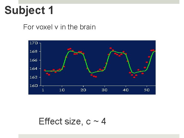
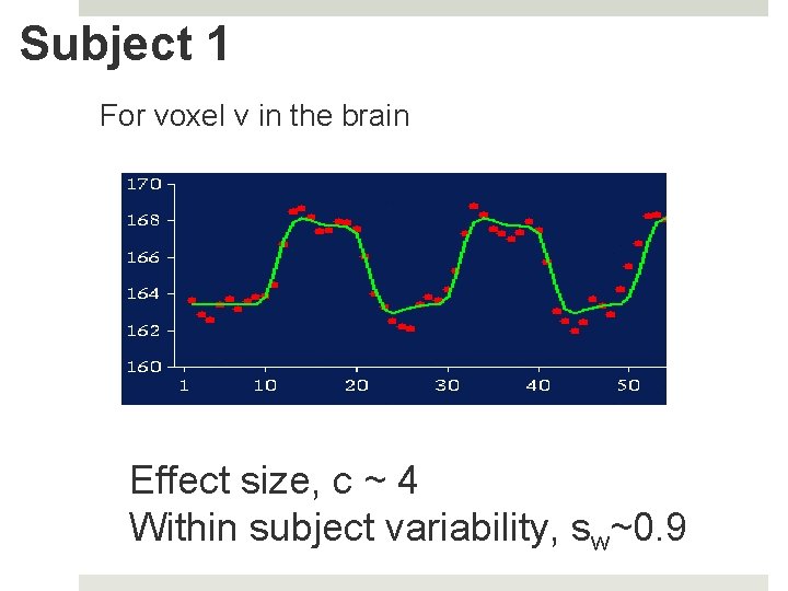
Subject 1 For voxel v in the brain Effect size, c ~ 4

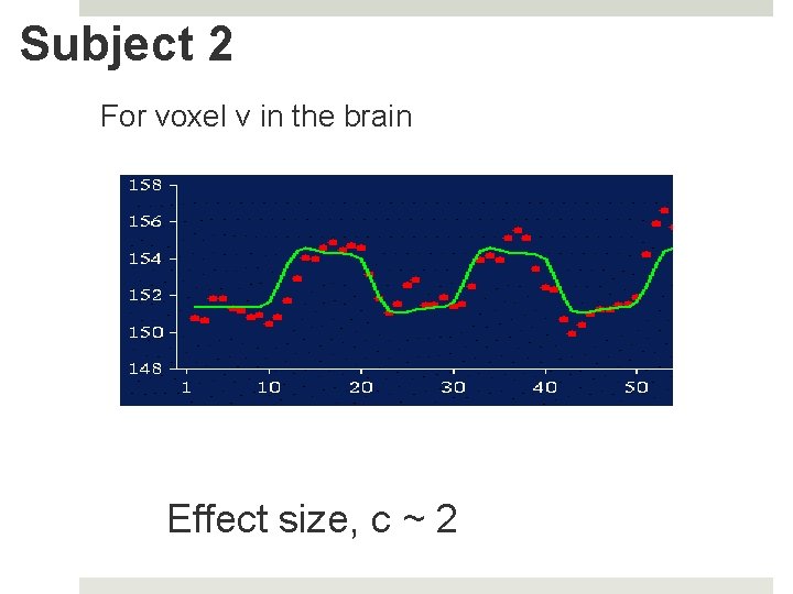
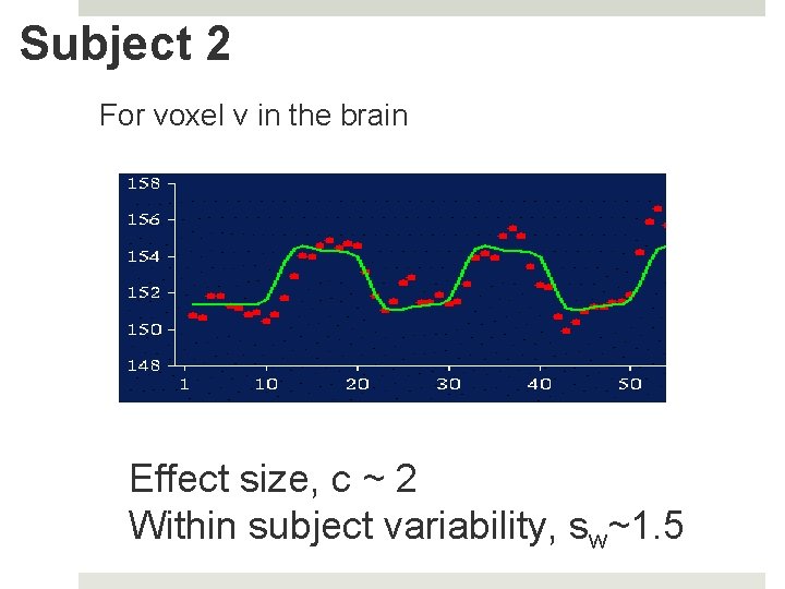
Subject 2 For voxel v in the brain Effect size, c ~ 2

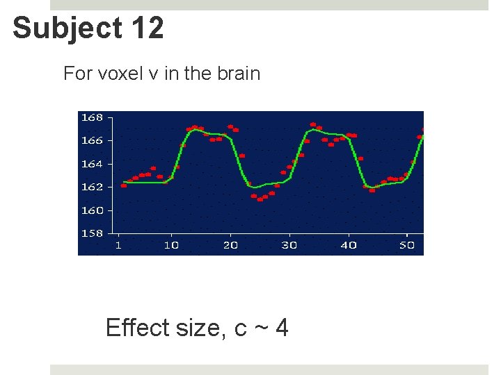
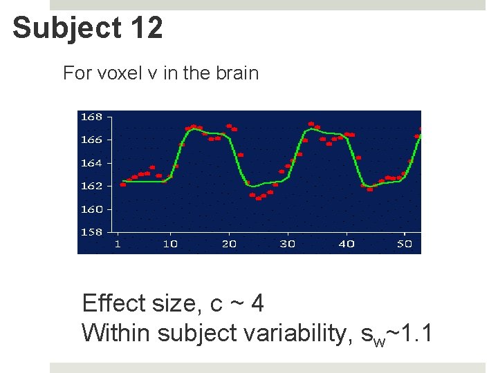
Subject 12 For voxel v in the brain Effect size, c ~ 4

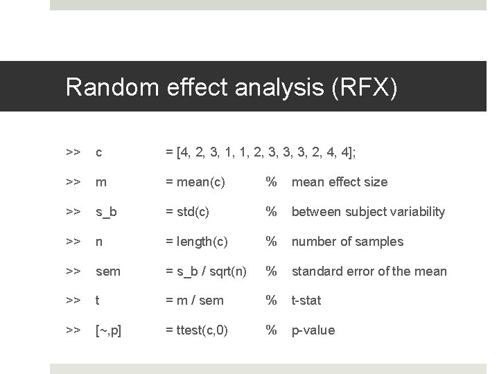
Random effect analysis (RFX) >> c = [4, 2, 3, 1, 1, 2, 3, 3, 3, 2, 4, 4]; >> m = mean(c) % mean effect size >> s_b = std(c) % between subject variability >> n = length(c) % number of samples >> sem = s_b / sqrt(n) % standard error of the mean >> t = m / sem % t-stat >> [~, p] = ttest(c, 0) % p-value

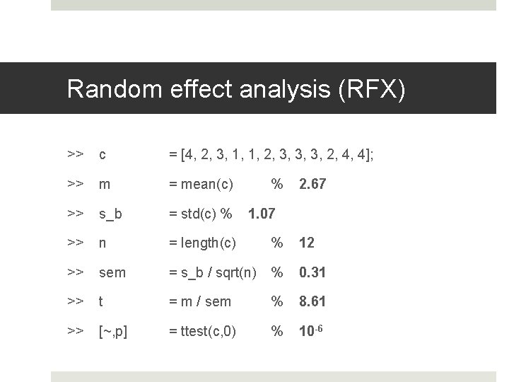
Random effect analysis (RFX) >> c = [4, 2, 3, 1, 1, 2, 3, 3, 3, 2, 4, 4]; >> m = mean(c) >> s_b = std(c) % >> n = length(c) % 12 >> sem = s_b / sqrt(n) % 0. 31 >> t = m / sem % 8. 61 >> [~, p] = ttest(c, 0) % 10 -6 % 2. 67 1. 07

Subject 1 For voxel v in the brain Effect size, c ~ 4 Within subject variability, sw~0. 9

Subject 2 For voxel v in the brain Effect size, c ~ 2 Within subject variability, sw~1. 5

Subject 12 For voxel v in the brain Effect size, c ~ 4 Within subject variability, sw~1. 1

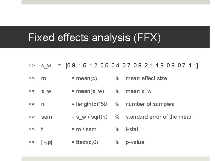
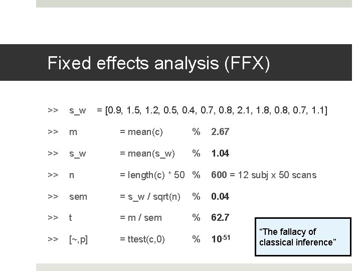
Fixed effects analysis (FFX) >> s_w = [0. 9, 1. 5, 1. 2, 0. 5, 0. 4, 0. 7, 0. 8, 2. 1, 1. 8, 0. 7, 1. 1] >> m = mean(c) % mean effect size >> s_w = mean(s_w) % mean s_w >> n = length(c)*50 % number of samples >> sem = s_w / sqrt(n) % standard error of the mean >> t = m / sem % t-stat >> [~, p] = ttest(c, 0) % p-value

Fixed effects analysis (FFX) >> s_w >> m = mean(c) % 2. 67 >> s_w = mean(s_w) % 1. 04 >> n = length(c) * 50 % 600 = 12 subj x 50 scans >> sem = s_w / sqrt(n) % 0. 04 >> t = m / sem % 62. 7 % 10 -51 >> [~, p] = [0. 9, 1. 5, 1. 2, 0. 5, 0. 4, 0. 7, 0. 8, 2. 1, 1. 8, 0. 7, 1. 1] = ttest(c, 0) “The fallacy of classical inference”

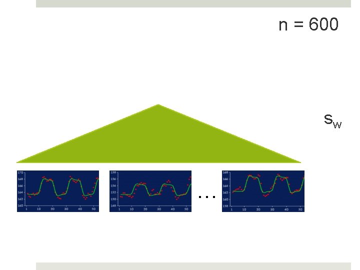
n = 600 sw …

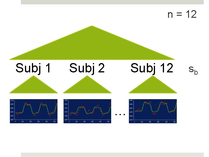
n = 12 Subj 1 Subj 2 Subj 12 … sb

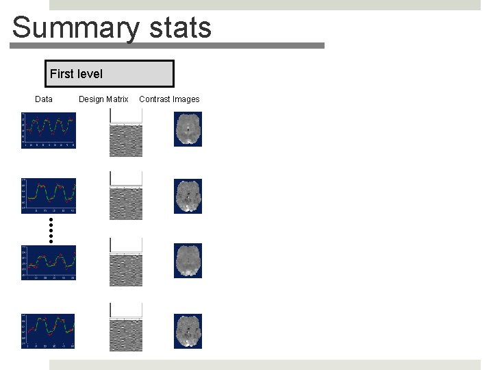
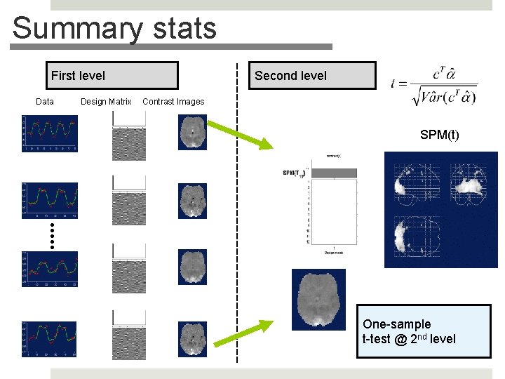
Summary stats First level Data Design Matrix Contrast Images

Summary stats First level Data Design Matrix Second level Contrast Images SPM(t) One-sample t-test @ 2 nd level

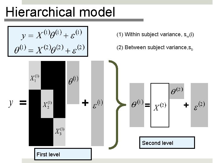
Hierarchical model (1) Within subject variance, sw(i) (2) Between subject variance, sb = + = Second level First level +

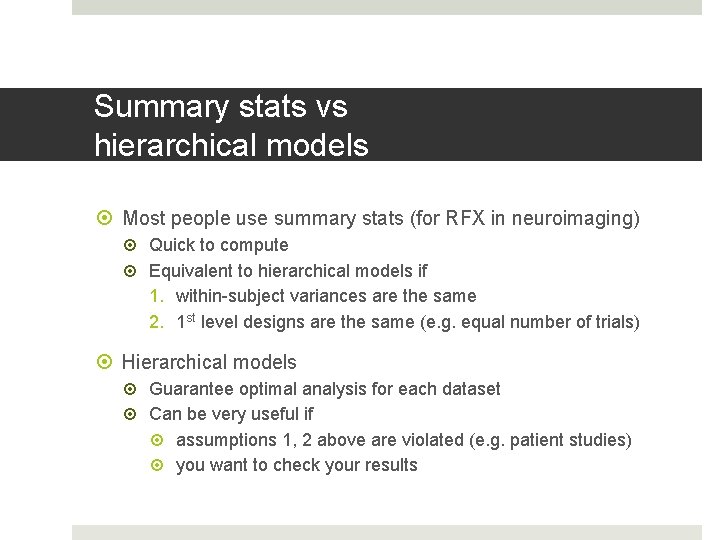
Summary stats vs hierarchical models Most people use summary stats (for RFX in neuroimaging) Quick to compute Equivalent to hierarchical models if 1. within-subject variances are the same 2. 1 st level designs are the same (e. g. equal number of trials) Hierarchical models Guarantee optimal analysis for each dataset Can be very useful if assumptions 1, 2 above are violated (e. g. patient studies) you want to check your results

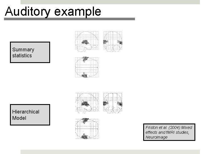
Auditory example Summary statistics Hierarchical Model Friston et al. (2004) Mixed effects and f. MRI studies, Neuroimage

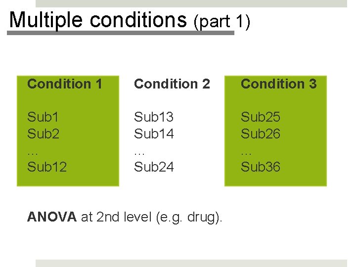
Multiple conditions (part 1) Condition 1 Condition 2 Condition 3 Sub 1 Sub 2. . . Sub 12 Sub 13 Sub 14. . . Sub 24 Sub 25 Sub 26. . . Sub 36 ANOVA at 2 nd level (e. g. drug).

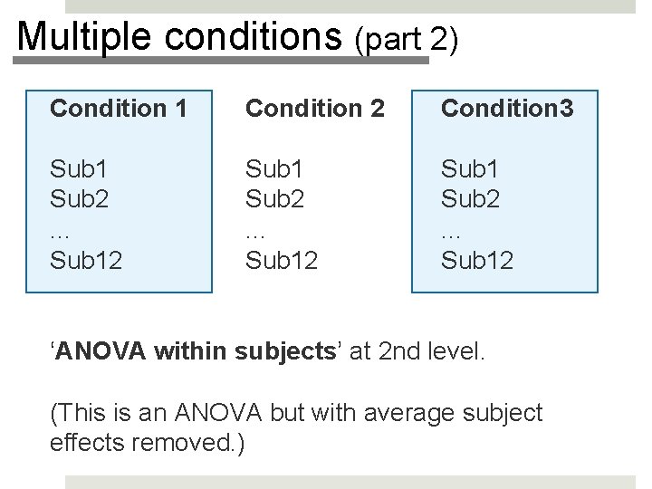
Multiple conditions (part 2) Condition 1 Condition 2 Condition 3 Sub 1 Sub 2. . . Sub 12 ‘ANOVA within subjects’ at 2 nd level. (This is an ANOVA but with average subject effects removed. )

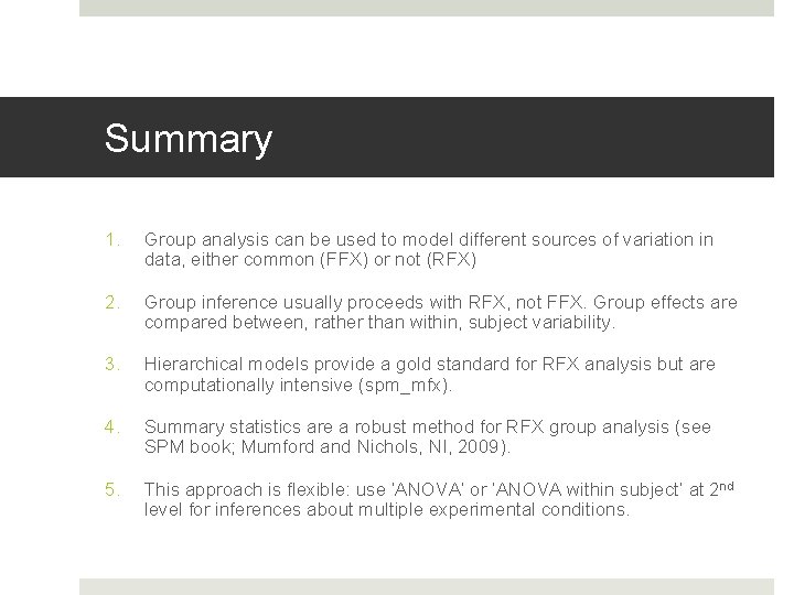
Summary 1. Group analysis can be used to model different sources of variation in data, either common (FFX) or not (RFX) 2. Group inference usually proceeds with RFX, not FFX. Group effects are compared between, rather than within, subject variability. 3. Hierarchical models provide a gold standard for RFX analysis but are computationally intensive (spm_mfx). 4. Summary statistics are a robust method for RFX group analysis (see SPM book; Mumford and Nichols, NI, 2009). 5. This approach is flexible: use ‘ANOVA’ or ‘ANOVA within subject’ at 2 nd level for inferences about multiple experimental conditions.