Group Analysis File afni 24Group Ana pdf Gang

Group Analysis File: afni 24_Group. Ana. pdf Gang Chen SSCC/NIMH/NIH/DHHS/USA/Earth

Program List • 3 dttest++ (GLM: one-, two-sample, paired t, between-subjects variables) • 3 d. MVM (generic AN(C)OVA) • 3 d. LME (sophisticated cases: missing data, within-subject covariates) • 3 d. MEMA (similar to 3 dttest++: measurement errors) • 3 d. ANOVA (one-way between-subject) • 3 d. ANOVA 2 (one-way within-subject, 2 -way between-subjects) • 3 d. ANOVA 3 (2 -way within-subject and mixed, 3 -way between-subjects) • 3 dttest (obsolete: one-sample, two-sample and paired t) • 3 d. Reg. Ana (obsolete: regression/correlation, covariates) • Group. Ana (obsolete: up to four-way ANOVA) • 3 d. ICC (intraclass correlation): prototype only • 3 d. ISC (intersubject correlation): prototype only -2 -

Preview of Coming Attractions • Concepts and terminology • Group analysis approaches o o GLM: 3 dttest++, 3 d. MEMA GLM, ANOVA, ANCOVA: 3 d. MVM LME: 3 d. LME Presumed vs. estimated HDR (i. e. , fixed vs. variable shape) • Miscellaneous o o o Issues with covariates Intra-Class Correlation (ICC) Inter-Subject Correlation (ISC) Goal = Give outline of AFNI capabilities in group analyses Decisions about complex situations require help https: //afni. nimh. nih. gov/afni/community/board -3 -

Why Group Analysis? • Reproducibility and generalization o Summarization o Generalization: from current results to population level o Typically 10 or more subjects per group o Individualized inferences: pre-surgical planning, lie detection, … • One model combining both steps (single subject and group)? o + Ideal: less information loss, more accurate inferences o - Historical o - Computationally unmanageable, and very hard to set up o - Data quality check at individual level -4 -

Simplest case • BOLD responses from a group of 20 subjects data: (β 1, β 2, …, β 20)=(1. 13, 0. 87, …, 0. 72) o mean: 0. 92 o standard deviation of the betas: 0. 40 or. 90 o Do we have strong evidence for the effect being nonzero? o • Statistical modeling perspective o Simplest GLM: one-sample t-test Statistical evidence - t-test: o summarization: b (dimensional), sd, and t (dimensionless) o -5 -

Terminology • Response/outcome variable: left-hand side of model Regression βi coefficients (plus measurement errors) o Structured: subjects, tasks, groups o • Explanatory variables: right-hand side of model Categorical (factors) vs quantitative (covariates) o Fixed- vs random-effects: conventional statistics o • Type of Models Univariate GLM: Student’s t-tests, regression, AN(C)OVA o Multivariate GLM: within-subject factors o LME: linear mixed-effects model o MEMA: mixed-effects multilevel analysis o BML (Bayesian multilevel model) o -6 -

Terminology: categorical vs quantitative • Factors Finite (small) number of levels: categories (coded by labels) o Within-subject (repeated-measures): tasks, conditions o Between-subjects o § § o patients/controls, genotypes, scanners/sites, handedness, … Each subject nested within a group Subjects: random-effects factor - measuring randomness § Of no intrinsic interest: random samples from a population • Quantitative variables numeric or continuous o age, IQ, reaction time, brain volume, … o 3 usages of “covariate” o No interest: § Qualitative (e. g. , scanner/site, groups) § Quantitative (e. g. , per subject amount of head motion) § Explanatory variable (e. g. , subject age, anxiety score) § -7 -

Terminology: fixed vs random • Fixed-effects variables o Of research interest § § o Modeled as constants, not random variables § o Visual vs auditory, age, … Unable to extend to something else Shared by all subjects Not exchangeable/replaceable or extendable to something else • Random-effects variables (mean + random part) o Of research interest? § § Subjects: random samples Trials, regions? Modeled as random variables: Gaussian distributions o Exchangeable, replaceable, generalizable o • Differentiations blurred under BML (Bayesian Multi-Level) -8 -

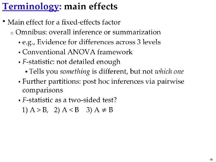
Terminology: interactions • Interaction effect between 2 or more factors o Omnibus: overall inference or summarization § § § o Conventional ANOVA framework F-statistic: not detailed enough to tell what specifically is happening Further partitions: post hoc inferences via pairwise comparisons 2 × 2 design: difference of difference § F-test for 2 x 2 interaction = t-test of (A 1 B 1 - A 1 B 2) - (A 2 B 1 - A 2 B 2) or (A 1 B 1 - A 2 B 1) - (A 1 B 2 - A 2 B 2) -10 -

Terminology • Interaction effect involving a quantitative variable o By default: linearity (age, modulation, …) § § o Controlling: misconception – e. g. , “covary out” age differences? or, Effect of interest Interaction between a factor and a quantitative variable -11 -

Terminology • Interaction effect involving a quantitative variable o Validity of linearity of b with (e. g. ) age § Nonlinear: difficult (too much freedom)! Polynomials? Theory-driven? -12 -

Example: 2 × 3 Mixed ANCOVA • Explanatory variables o o Factor A (Group): 2 levels (patient and control) Factor B (Condition): 3 levels (pos, neg, neu – emotional words) Factor S (Subject): 15 ASD children and 15 healthy controls Quantitative covariate: Age • Piecemeal: multiple t-tests – too tedious o o o Group comparison + age effect Pairwise comparisons among three conditions § Assumption: same age effect across conditions Difficulties with t-tests § Main effect of Condition: 3 levels plus age? § Interaction between Group and Condition § Age effect across three conditions? -13 -

Classical ANOVA: 2 × 3 Mixed ANOVA (no covariate) o Factor A (Group): 2 levels (patient and control) o Factor B (Condition): 3 levels (pos, neg, neu) o Factor S (Subject): 15 ASD children and 15 healthy controls o Covariate (Age): cannot be modeled; no correction for sphericity violation Different denominators 3 d. ANOVA 3 –type 5 (equal # of subjects across groups) -14 -

Univariate GLM: 2 x 3 mixed ANOVA o Group: 2 levels (patient and control) o Condition: 3 levels (pos, neg, neu) o Subject: 3 ASD children and 3 healthy controls b X Difficult to incorporate covariates • Broken orthogonality of matrix No correction for sphericity violation a d -15 -

Univariate GLM: problematic implementations (in some other software we won’t name) Two-way mixed ANOVA Between-subjects Factor A (Group): 2 levels (patient, control) Within-subject Factor B (Condition): 3 levels (pos, neg, neu) 1) Omnibus tests Correct Incorrect 2) Post hoc tests (contrasts) - Incorrect t-tests for factor A due to incorrect denominator - Incorrect t-tests for factor B or interaction effect AB when weights do not add up to 0 -16 -

Univariate GLM: problematic implementations Two-way repeated-measures ANOVA Within-subjects Factor A (Object): 2 levels (house, face) Within-subject Factor B (Condition): 3 levels (pos, neg, neu) 1) Omnibus tests Correct Incorrect 2) Post hoc tests (contrasts) - Incorrect t-tests for both factors A and B due to incorrect denominator - Incorrect t-tests for interaction effect AB if weights don’t add up to 0 -17 -

Better Approach: Multivariate GLM o Group: 2 levels (patient and control) o Condition: 3 levels (pos, neg, neu) o Subject: 3 ASD children and 3 healthy controls o Age: quantitative covariate Βn×m = Xn×q Aq×m + Dn×m B B Data = betas X A D Model = Design matrix = Main Effect & Group Coding & Covariate Fit Parameters (to be computed) Residuals -18 -

MVM Implementation in AFNI • Program 3 d. MVM – generalize multi-way ANCOVA, and more o No dummy coding needed! o Symbolic coding for variables and post hoc testing Variable types Post hoc tests Data layout

MVM General Linear Tests – besides main effects o Symbolic coding for variables and post hoc testing o o o -bs. VARS ‘Grp*Age’ shows 2 between subjects variables o -q. Vars ‘Age’ shows one is quantitative (numbers) o So the other one Grp is categorical (labels) o -ws. Vars ‘Cond’ shows 1 within subjects variable (categorical) o Potential values for all variables collated from data table GLT #3 “Grp : 1*Pat Cond : 1*Pos -1*Neg” o Within the Grp variable, select the Pat mean effect o Within the Cond variable, select the difference between the Pos and Neg mean effects o Age is not specified, so test will be carried out on the effects regressed to the Age center (for each Grp) GLT #4 “Grp : 1*Pat Age : ” tests the slope of the betas w. r. t. Age for Patients (averaged across Cond values)

Improvement 1: precision information • Conventional approach: βs as response variable o Assumptions § § o no measurement errors all subjects have same precision All subjects are treated equally (have the same randomness) • More precise method: estimated βs plus precision estimates o o o t-statistic contains precision (t = β / SEM(β) ) βs and their t-stats as input βs weighted based on precision Only available for simple GLM types: 3 d. MEMA Regions with substantial cross-subject variability • Best approach: combining all subjects in one big super-model o Currently not feasible -21 -

One group: Example • 3 dttest++: β as input only 3 dttest++ –prefix Vis -mask+tlrc -zskip -set. A ‘FP+tlrc[Vrel#0_Coef]’ ’FR+tlrc[Vrel#0_Coef]’ …… Voxel value = 0 treated it as missing ’GM+tlrc[Vrel#0_Coef]’ • 3 d. MEMA: β and t-statistic as input 3 d. MEMA –prefix Vis. MEMA -mask+tlrc -set. A Vis FP ’FP+tlrc[Vrel#0_Coef]’ ’FP+tlrc[Vrel#0_Tstat]’ FR ’FR+tlrc[Vrel#0_Coef]’ ’FR+tlrc[Vrel#0_Tstat]’ …… GM ’GM+tlrc[Vrel#0_Coef]’ ’GM+tlrc[Vrel#0_Tstat]’ -missing_data 0 Voxel value = 0 treated it as missing -22 -

Paired comparison: Example • 3 dttest++: comparing two conditions 3 dttest++ –prefix Vis_Aud -mask+tlrc –paired -zskip -set. A ’FP+tlrc[Vrel#0_Coef]’ ’FR+tlrc[Vrel#0_Coef]’ …… ’GM+tlrc[Vrel#0_Coef]’ -set. B ’FP+tlrc[Arel#0_Coef]’ ’FR+tlrc[Arel#0_Coef]’ …… ’GM+tlrc[Arel#0_Coef]’ -23 -

Paired Comparison: Example • 3 d. MEMA: accounting for differential accuracy (among βs) o Contrast as input 3 d. MEMA –prefix Vis_Aud_MEMA -mask+tlrc -missing_data 0 -set. A Vis-Aud FP ’FP+tlrc[Vrel-Arel#0_Coef]’ ’FP+tlrc[Vrel-Arel#0_Tstat]’ FR ’FR+tlrc[Vrel-Arel#0_Coef]’ ’FR+tlrc[Vrel-Arel#0_Tstat]‘ …… GM ’GM+tlrc[Vrel-Arel#0_Coef]’’GM+tlrc[Vrel-Arel#0_Tstat]’ -24 -

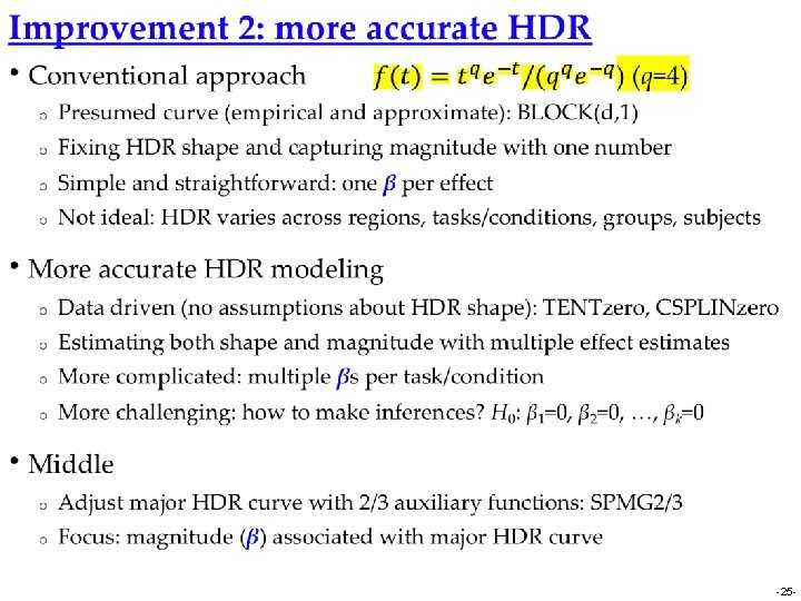
Improvement 2: more accurate HDR • Group analysis with HDR estimates: TENTzero, CSPLINzero o NHST: H 0: β 1=0, β 2=0, …, βk=0 [all responses in HRF = zero] o Area under curve (AUC) approach o § Reduce HRF to one number: use area as magnitude approximation § Ignore shape subtleties § Shape information loss: (undershoot, peak location/width) Better approach: maintaining shape integrity § Take individual βs to group analysis (MVM) § One group with one condition: 3 d. LME § Other scenarios: treat βs as levels of a factor (e. g. , Time) - 3 d. MVM ** Task or group effect: F-stat for interaction between task group and Time, complemented with main effect for task/group (AUC) Chen et al. (2015). Detecting the subtle shape differences in hemodynamic responses at the group level. Front. Neurosci. , 26 October 2015. -26 -

Improvement 2: more accurate HDR • 2 groups (children, adults), 2 conditions (congruent, incongruent), 1 quantitative covariate (age) • 2 methods: HRF modeled by 10 (tents) and 3 (SPMG 3) bases • Effect of interaction: interaction group: condition – 3 d. MVM -27 -

Improvement 2: more accurate HDR • Advantages of ESM over FSM o o More likely to detect HDR shape subtleties Visual verification of HDR signature shape (vs. relying significance testing: p-values) Study: Adults/Children with Congruent/Incongruent stimuli (2× 2) -28 -

Dealing with quantitative variables • Reasons to consider a covariate o Effect of interest: variability of response with some subject parameter o Model improvement: accounting for data variability with plausible cause o But you don’t particularly care about this effect per se • Frameworks o ANCOVA: between-subjects factor (e. g. , group) + quantitative variable o Broader frameworks: regression, GLM, MVM, LME, BML o Assumptions: linearity, homogeneity of slopes (interaction) • Interpretations o Effect of interest: slope, rate, marginal effect o Regress/covariate out x? (e. g. , head motion at individual level) o “Controlling x at …”, “holding x constant”: centering -29 -

Quantitative variables: centering • Model o o α 1, α 2 - slope α 0 – intercept: group effect when x=0 Not necessarily meaningful by itself § Linearity may not hold over large ranges of x 1 or x 2 § Centering covariates for interpretability § Mean or median centering? § • When a factor is involved o Complicated decision: within-level or grand centering https: //afni. nimh. nih. gov/pub/dist/doc/htmldoc/STATISTICS/center. html -30 -

A Useful Article about Covariates • • • Miller GM and Chapman JP. Misunderstanding analysis of covariance J Abnormal Psych 110: 40 -48 (2001) http: //dx. doi. org/10. 1037/0021 -843 X. 110. 1. 40 http: //psycnet. apa. org/journals/abn/110/1/40. pdf -31 -

Intra. Class Correlation (ICC) • Reliability (consistency, agreement/reproducibility) across two or more measurements of same/similar condition/task o sessions, scanners, sites, studies, twins o o Classic example (Shrout and Fleiss, 1979): n targets are rated by k raters Relationship with Pearson correlation § § Pearson correlation: two different types of measure: e. g. , BOLD response vs. RT § how much does one measurement type “explain” the other? ICC: same measurement type – how reliable are the results? Modeling frameworks: ANOVA, LME 3 types of ICC: ICC(1, 1), ICC(2, 1), ICC(3, 1) – one-, two-way random- and mixed-effects ANOVA • Whole-brain voxel-level ICC o o ICC(2, 1): 3 d. LME –ICC or 3 d. LME –ICCb 3 d. ICC: ICC(1, 1), ICC(2, 1) and ICC(3, 1) Chen et al. (2017), Human Brain Mapping 39(3) DOI: 10. 1002/hbm. 23909 -32 -

Naturalistic scanning • Subjects view a natural scene during scanning o Visuoauditory movie clip (e. g. , http: //studyforrest. org/) o Music, speech, games, … • Duration: a few minutes (at least) or more • Close to naturalistic settings: minimally manipulated • Effect of interest: intersubject correlation (ISC) – 3 d. Tcorrelate • Calculates correlation coefficient between voxel time series between subjects • Usual input is errts dataset after pre-processing to “correct” for motion, align to template space, et cetera o Extent of synchronization (“entrainment”) o Or of common response in that voxel/region across subjects to whatever they were experiencing • Whole-brain voxel-wise group analysis of these voxel-wise intersubject correlations: 3 d. ISC -33 -

ISC group analysis • Voxel-wise ISC matrix (usually Fisher/arctanh-transformed) o One group o Two groups § Within-group ISC: R 11, R 22 § Inter-group ISC: R 21 § 3 group comparisons: R 11 vs R 22, R 11 vs R 21, R 22 vs R 21 -34 -

Complexity of ISC analysis • 2 ISC values associated with a common subject are correlated with each other: 5 subjects ⇢ 5 x 4/2 = 10 ISC values • i. e. , random fluctuations in inter-subject correlations are correlated • ρ ≠ 0 (unknown) characterizes non-independent relationship • Challenge: how to handle this irregular correlation matrix? -35 -

ISC: LME approach • Modeling via effect partitioning: crossed random-effects LME cross-subject within-subject • Charactering the relatedness among ISCs via LME Chen et al, 2016. Untangling the Relatedness among Correlations, Part II: Inter-Subject Correlation Group Analysis through Linear Mixed-Effects Modeling. Neuroimage. Neuro. Image 147: 825 -840 -36 -

Summary • Concepts and terminology • Group analysis approaches o o GLM: 3 dttest++, 3 d. MEMA GLM, ANOVA, ANCOVA: 3 d. MVM LME: 3 d. LME Presumed vs. estimated HDR • Miscellaneous o o o Issues with covariates Intra-Class Correlation (ICC) Inter-Subject Correlation (ISC) -37 -

Program List • 3 dttest++ (GLM: one-, two-sample, paired t, between-subjects variables) • 3 d. MVM (generic AN(C)OVA) • 3 d. LME (sophisticated cases: missing data, within-subject covariates) • 3 d. MEMA (similar to 3 dttest++: measurement errors) • 3 d. ANOVA (one-way between-subject) • 3 d. ANOVA 2 (one-way within-subject, 2 -way between-subjects) • 3 d. ANOVA 3 (2 -way within-subject and mixed, 3 -way between-subjects) • 3 dttest (obsolete: one-sample, two-sample and paired t) • 3 d. Reg. Ana (obsolete: regression/correlation, covariates) • Group. Ana (obsolete: up to four-way ANOVA) • 3 d. ICC (intraclass correlation): prototype only • 3 d. ISC (intersubject correlation): prototype only -38 -