Group Analysis with FourWay ANOVA in AFNI Gang

- Slides: 1

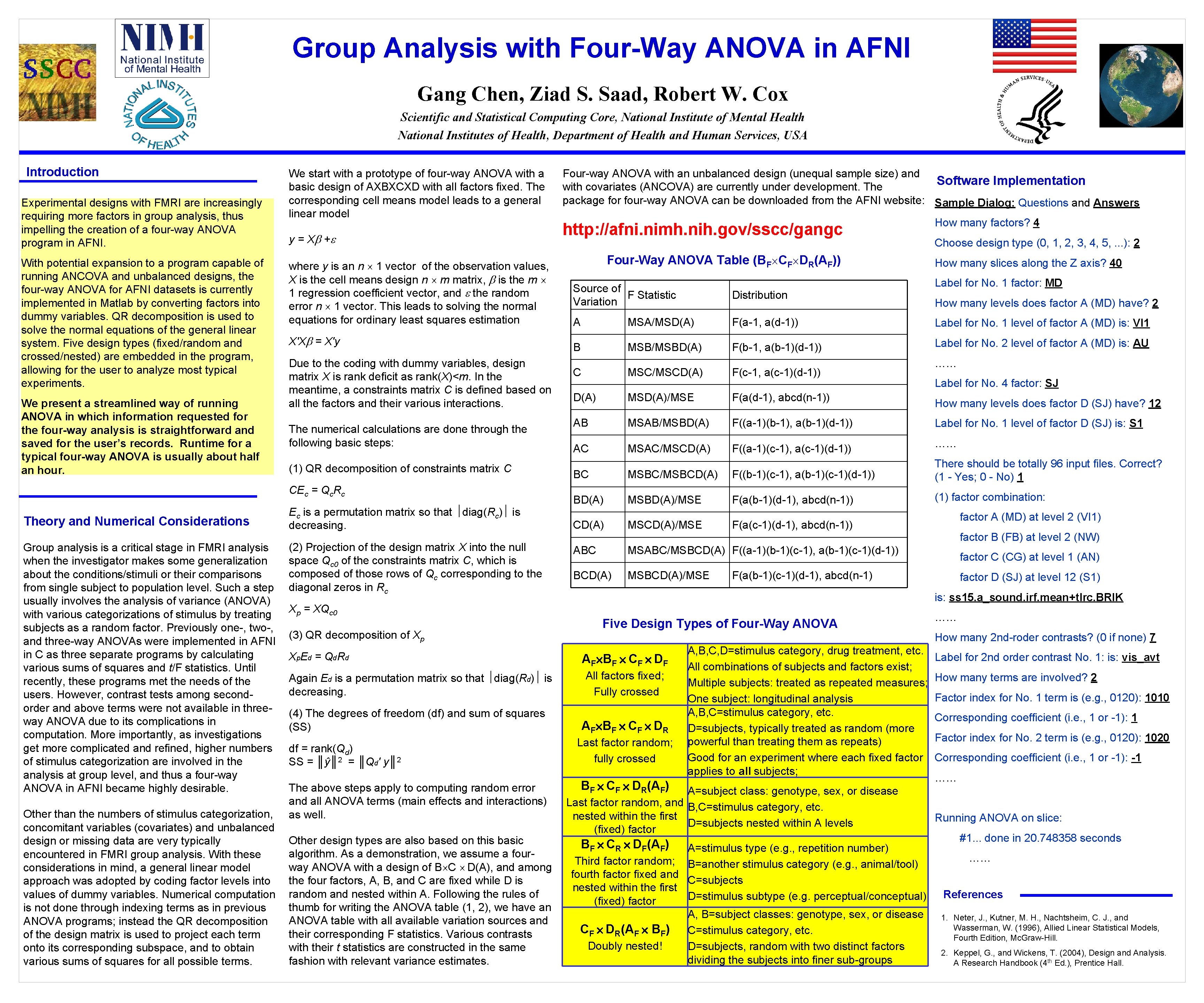
Group Analysis with Four-Way ANOVA in AFNI Gang Chen, Ziad S. Saad, Robert W. Cox Scientific and Statistical Computing Core, National Institute of Mental Health National Institutes of Health, Department of Health and Human Services, USA Introduction Experimental designs with FMRI are increasingly requiring more factors in group analysis, thus impelling the creation of a four-way ANOVA program in AFNI. With potential expansion to a program capable of running ANCOVA and unbalanced designs, the four-way ANOVA for AFNI datasets is currently implemented in Matlab by converting factors into dummy variables. QR decomposition is used to solve the normal equations of the general linear system. Five design types (fixed/random and crossed/nested) are embedded in the program, allowing for the user to analyze most typical experiments. We present a streamlined way of running ANOVA in which information requested for the four-way analysis is straightforward and saved for the user’s records. Runtime for a typical four-way ANOVA is usually about half an hour. We start with a prototype of four-way ANOVA with a basic design of AXBXCXD with all factors fixed. The corresponding cell means model leads to a general linear model y = X + where y is an n 1 vector of the observation values, X is the cell means design n m matrix, is the m 1 regression coefficient vector, and the random error n 1 vector. This leads to solving the normal equations for ordinary least squares estimation X'X = X'y Due to the coding with dummy variables, design matrix X is rank deficit as rank(X)<m. In the meantime, a constraints matrix C is defined based on all the factors and their various interactions. The numerical calculations are done through the following basic steps: (1) QR decomposition of constraints matrix C CEc = Qc. Rc Theory and Numerical Considerations Group analysis is a critical stage in FMRI analysis when the investigator makes some generalization about the conditions/stimuli or their comparisons from single subject to population level. Such a step usually involves the analysis of variance (ANOVA) with various categorizations of stimulus by treating subjects as a random factor. Previously one-, two-, and three-way ANOVAs were implemented in AFNI in C as three separate programs by calculating various sums of squares and t/F statistics. Until recently, these programs met the needs of the users. However, contrast tests among secondorder and above terms were not available in threeway ANOVA due to its complications in computation. More importantly, as investigations get more complicated and refined, higher numbers of stimulus categorization are involved in the analysis at group level, and thus a four-way ANOVA in AFNI became highly desirable. Other than the numbers of stimulus categorization, concomitant variables (covariates) and unbalanced design or missing data are very typically encountered in FMRI group analysis. With these considerations in mind, a general linear model approach was adopted by coding factor levels into values of dummy variables. Numerical computation is not done through indexing terms as in previous ANOVA programs; instead the QR decomposition of the design matrix is used to project each term onto its corresponding subspace, and to obtain various sums of squares for all possible terms. Ec is a permutation matrix so that diag(Rc) is decreasing. (2) Projection of the design matrix X into the null space Qc 0 of the constraints matrix C, which is composed of those rows of Qc corresponding to the diagonal zeros in Rc Xp = XQc 0 (3) QR decomposition of Xp X p. E d = Q d. R d Again Ed is a permutation matrix so that diag(Rd) is decreasing. (4) The degrees of freedom (df) and sum of squares (SS) df = rank(Qd) SS = ║ŷ║ 2 = ║Qd' y║ 2 The above steps apply to computing random error and all ANOVA terms (main effects and interactions) as well. Other design types are also based on this basic algorithm. As a demonstration, we assume a fourway ANOVA with a design of B C D(A), and among the four factors, A, B, and C are fixed while D is random and nested within A. Following the rules of thumb for writing the ANOVA table (1, 2), we have an ANOVA table with all available variation sources and their corresponding F statistics. Various contrasts with their t statistics are constructed in the same fashion with relevant variance estimates. Four-way ANOVA with an unbalanced design (unequal sample size) and Software Implementation with covariates (ANCOVA) are currently under development. The package for four-way ANOVA can be downloaded from the AFNI website: Sample Dialog: Questions and Answers http: //afni. nimh. nih. gov/sscc/gangc Four-Way ANOVA Table (BF CF DR(AF)) How many factors? 4 Choose design type (0, 1, 2, 3, 4, 5, . . . ): 2 How many slices along the Z axis? 40 Label for No. 1 factor: MD Source of F Statistic Variation Distribution A MSA/MSD(A) F(a-1, a(d-1)) Label for No. 1 level of factor A (MD) is: VI 1 B MSB/MSBD(A) F(b-1, a(b-1)(d-1)) Label for No. 2 level of factor A (MD) is: AU How many levels does factor A (MD) have? 2 …… C MSC/MSCD(A) F(c-1, a(c-1)(d-1)) D(A) MSD(A)/MSE F(a(d-1), abcd(n-1)) AB MSAB/MSBD(A) F((a-1)(b-1), a(b-1)(d-1)) Label for No. 1 level of factor D (SJ) is: S 1 F((a-1)(c-1), a(c-1)(d-1)) …… AC MSAC/MSCD(A) Label for No. 4 factor: SJ How many levels does factor D (SJ) have? 12 BC MSBC/MSBCD(A) F((b-1)(c-1), a(b-1)(c-1)(d-1)) There should be totally 96 input files. Correct? (1 - Yes; 0 - No) 1 BD(A) MSBD(A)/MSE F(a(b-1)(d-1), abcd(n-1)) (1) factor combination: CD(A) MSCD(A)/MSE ABC MSABC/MSBCD(A) F((a-1)(b-1)(c-1), a(b-1)(c-1)(d-1)) BCD(A) MSBCD(A)/MSE factor A (MD) at level 2 (VI 1) F(a(c-1)(d-1), abcd(n-1)) factor B (FB) at level 2 (NW) factor C (CG) at level 1 (AN) F(a(b-1)(c-1)(d-1), abcd(n-1) factor D (SJ) at level 12 (S 1) is: ss 15. a_sound. irf. mean+tlrc. BRIK Five Design Types of Four-Way ANOVA …… How many 2 nd-roder contrasts? (0 if none) 7 AF BF CF DF All factors fixed; Fully crossed AF BF CF DR Last factor random; fully crossed A, B, C, D=stimulus category, drug treatment, etc. All combinations of subjects and factors exist; Multiple subjects: treated as repeated measures; One subject: longitudinal analysis A, B, C=stimulus category, etc. D=subjects, typically treated as random (more powerful than treating them as repeats) Good for an experiment where each fixed factor applies to all subjects; BF CF DR(AF) A=subject class: genotype, sex, or disease Last factor random, and B, C=stimulus category, etc. nested within the first D=subjects nested within A levels (fixed) factor BF CR DF(AF) A=stimulus type (e. g. , repetition number) Third factor random; B=another stimulus category (e. g. , animal/tool) fourth factor fixed and C=subjects nested within the first D=stimulus subtype (e. g. perceptual/conceptual) (fixed) factor A, B=subject classes: genotype, sex, or disease CF DR(AF BF) C=stimulus category, etc. Doubly nested! D=subjects, random with two distinct factors dividing the subjects into finer sub-groups Label for 2 nd order contrast No. 1: is: vis_avt How many terms are involved? 2 Factor index for No. 1 term is (e. g. , 0120): 1010 Corresponding coefficient (i. e. , 1 or -1): 1 Factor index for No. 2 term is (e. g. , 0120): 1020 Corresponding coefficient (i. e. , 1 or -1): -1 …… Running ANOVA on slice: #1. . . done in 20. 748358 seconds …… References 1. Neter, J. , Kutner, M. H. , Nachtsheim, C. J. , and Wasserman, W. (1996), Allied Linear Statistical Models, Fourth Edition, Mc. Graw-Hill. 2. Keppel, G. , and Wickens, T. (2004), Design and Analysis. A Research Handbook (4 th Ed. ), Prentice Hall.