Gait recognition under nonstandard circumstances Kjetil Holien Disposition

Gait recognition under nonstandard circumstances Kjetil Holien

Disposition • • Research questions Introduction Gait as a biometric feature Analysis Experiment setup Results Conclusion Questions 1/27

Research questions • Main research questions: – To what extent is it possible to recognize a person under different circumstances? – Do the different circumstances have any common features? • Sub research question: – Do people walk in the same way given the same circumstances? 2/27

Introduction • Authentication can occur in three ways: – Something you know, password or PIN code. – Something you has, key or smartcard. – Something you are, biometrics. • Biometrics are divided into: – Physiological: properties that normally do not change, fingerprints and iris. – Behavioral: properties that are learned, such as signature and gait. 3/27

Gait as a biometric feature Three main approaches: – Machine Vision based. – Floor Sensor based. – Wearable Sensor based (our approach). 4/27

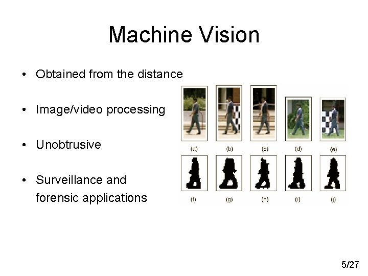
Machine Vision • Obtained from the distance • Image/video processing • Unobtrusive • Surveillance and forensic applications 5/27

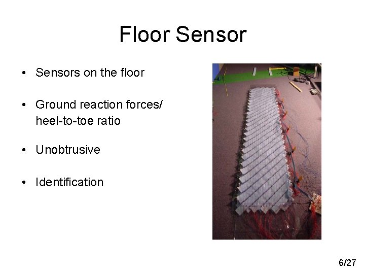
Floor Sensor • Sensors on the floor • Ground reaction forces/ heel-to-toe ratio • Unobtrusive • Identification 6/27

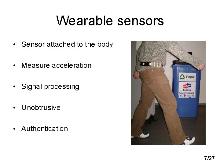
Wearable sensors • Sensor attached to the body • Measure acceleration • Signal processing • Unobtrusive • Authentication 7/27

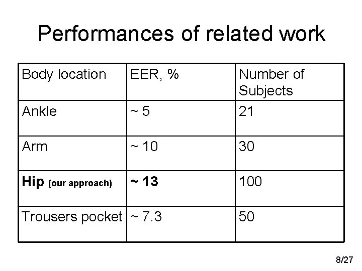
Performances of related work Body location EER, % Ankle ~5 Number of Subjects 21 Arm ~ 10 30 Hip (our approach) ~ 13 100 Trousers pocket ~ 7. 3 50 8/27

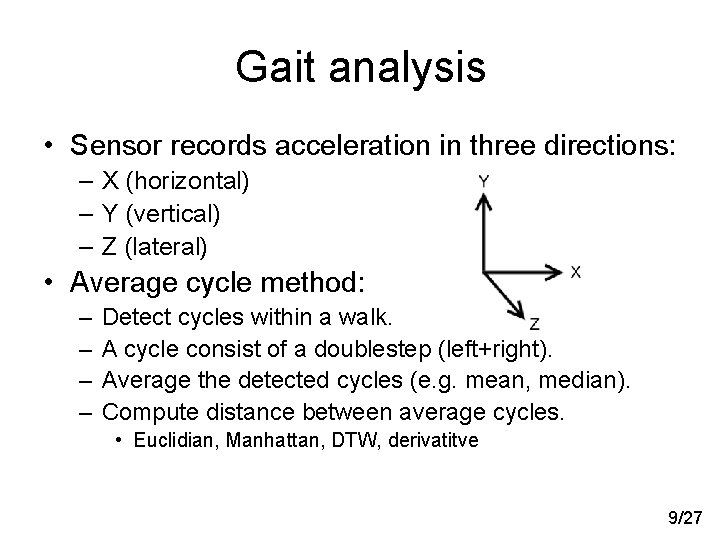
Gait analysis • Sensor records acceleration in three directions: – X (horizontal) – Y (vertical) – Z (lateral) • Average cycle method: – – Detect cycles within a walk. A cycle consist of a doublestep (left+right). Average the detected cycles (e. g. mean, median). Compute distance between average cycles. • Euclidian, Manhattan, DTW, derivatitve 9/27

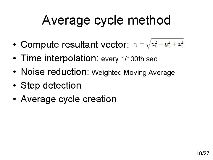
Average cycle method • • • Compute resultant vector: Time interpolation: every 1/100 th sec Noise reduction: Weighted Moving Average Step detection Average cycle creation 10/27

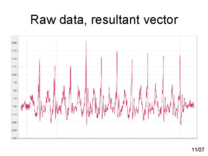
Raw data, resultant vector 11/27

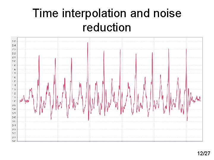
Time interpolation and noise reduction 12/27

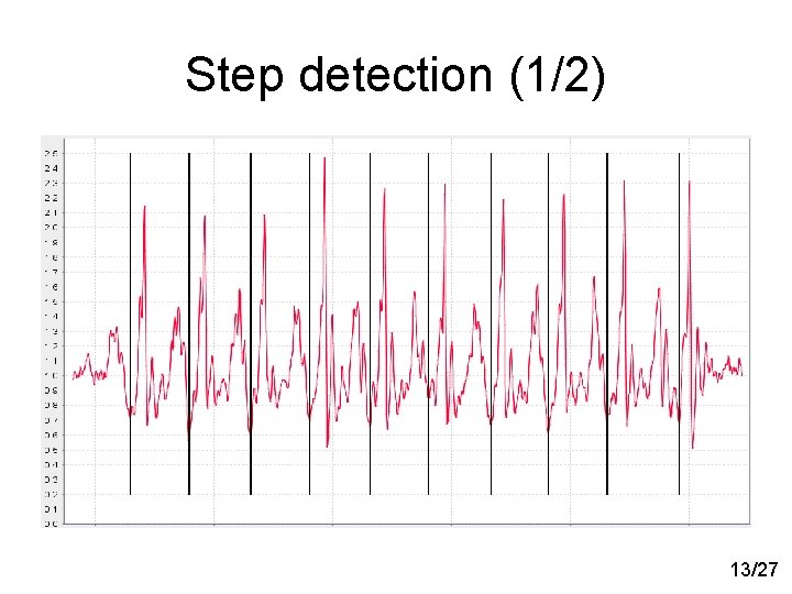
Step detection (1/2) 13/27

Step detection (2/2) • Consist of several sub-phases: – – Estimate cycle length Indicate amplitude details Detect starting location Detect rest of the steps 14/27

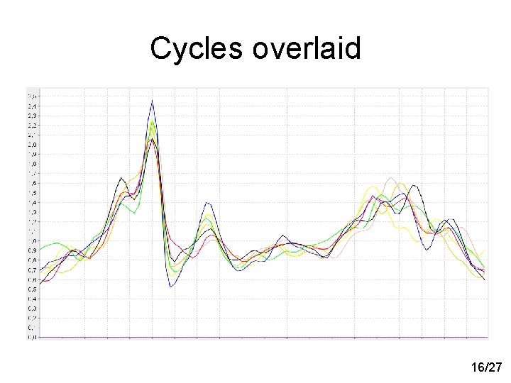
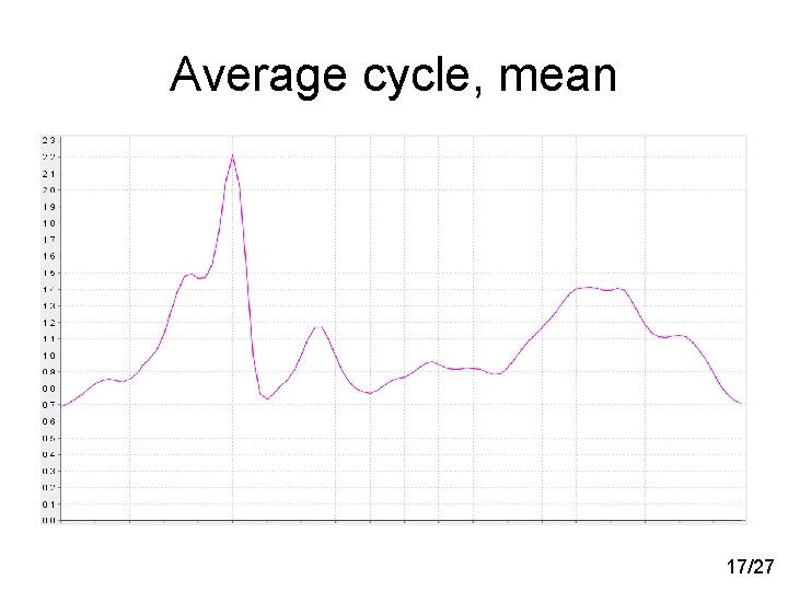
Creation of average cycle • Pre-processing methods: – – – Normalize to 100 samples Adjust acceleration Align maximum points Normalize amplitude Skip irregular cycles • Create average cycle: – – Mean Median Trimmed Mean Dynamic Time Warping 15/27

Cycles overlaid 16/27

Average cycle, mean 17/27

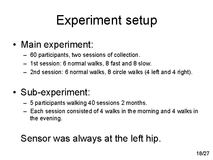
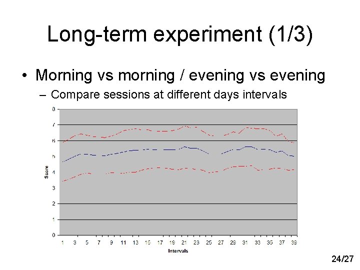
Experiment setup • Main experiment: – 60 participants, two sessions of collection. – 1 st session: 6 normal walks, 8 fast and 8 slow. – 2 nd session: 6 normal walks, 8 circle walks (4 left and 4 right). • Sub-experiment: – 5 participants walking 40 sessions 2 months. – Each session consisted of 4 walks in the morning and 4 walks in the evening. Sensor was always at the left hip. 18/27

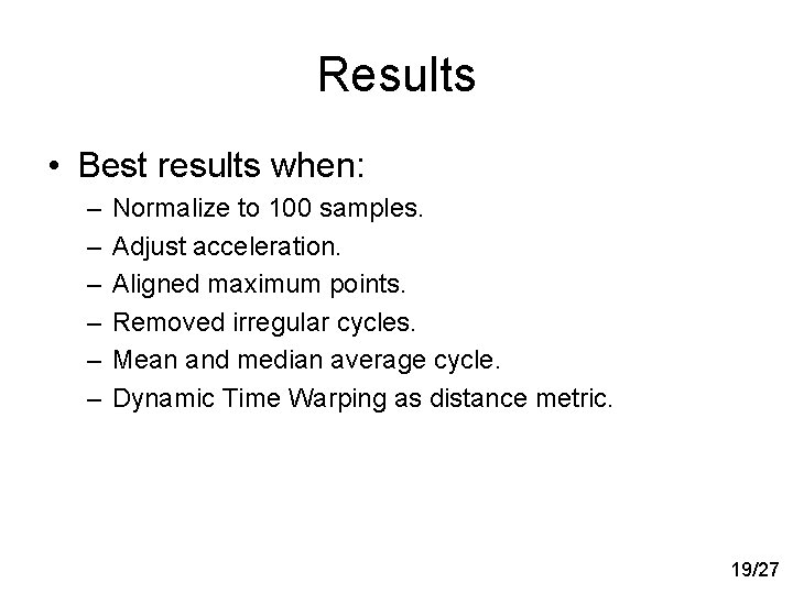
Results • Best results when: – – – Normalize to 100 samples. Adjust acceleration. Aligned maximum points. Removed irregular cycles. Mean and median average cycle. Dynamic Time Warping as distance metric. 19/27

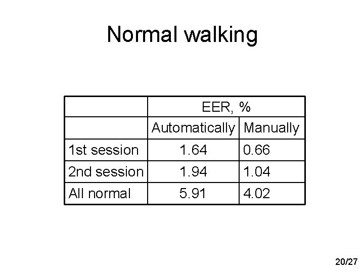
Normal walking EER, % Automatically Manually 1 st session 1. 64 0. 66 2 nd session 1. 94 1. 04 All normal 5. 91 4. 02 20/27

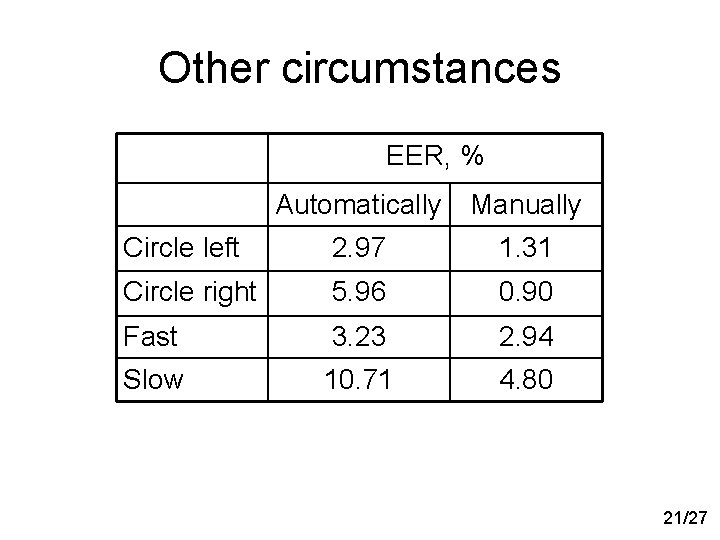
Other circumstances EER, % Automatically Manually Circle left 2. 97 1. 31 Circle right 5. 96 0. 90 Fast 3. 23 2. 94 Slow 10. 71 4. 80 21/27

All circumstances • Normal vs other circumstances – EER between 15 -30% • Multi-template – 1 template for each circumstance, the others as input – EER = 5. 05% 22/27

Common features • Cycle length: – – Normal: [95. . 125], average of 109 samples Fast: [80. . 110], average of 96 samples Slow: [110. . 180], average of 137 samples Circle same as normal • Amplitudes related to cycle length 23/27

Long-term experiment (1/3) • Morning vs morning / evening vs evening – Compare sessions at different days intervals 24/27

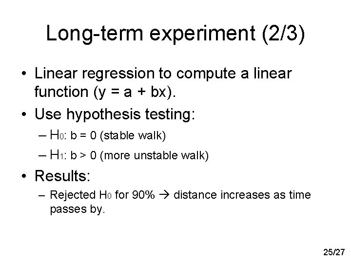
Long-term experiment (2/3) • Linear regression to compute a linear function (y = a + bx). • Use hypothesis testing: – H 0: b = 0 (stable walk) – H 1: b > 0 (more unstable walk) • Results: – Rejected H 0 for 90% distance increases as time passes by. 25/27

Long-term experiment (3/3) • Morning vs evening (same day) and evening vs the consecutive morning – No difference in the average scores. – Between 30% and 70% increase compared with 1 day interval scores. 26/27

Conclusion • Extremely good EER when comparing the circumstance with itself. • Different circumstances seems to be distinct hard to transform X to normal. • Good results when using a multi-template solution. • Gait seems to be unstable to some extent need a dynamic template. 27/27

Questions? Thanks for listening!