Fourth German Stata Users Group Meeting New Tools

Fourth German Stata Users Group Meeting New Tools for Evaluating the Results of Cluster Analyses Hilde Schaeper Higher Education Information System (HIS), Hannover/Germany schaeper@his. de Mannheim, March 31 st, 2006

Main features of cluster analysis New Tools for Evaluating the Results of Cluster Analyses 1

Steps and decisions in cluster analysis I Selection of a sample (outliers may influence the results) II Selection and transformation of variables (irrelevant and correlated variables can bias the classification; cluster analysis requires the variables to have equal scales) III Choice of the basic approach (in particular: agglomerative hierarchical vs. partitioning cluster analysis) IV Choice of a particular clustering technique V Selection of a dissimilarity or similarity measure (depends partly on the measurement level of the variables and the clustering technique chosen) VI Choice of the initial partition in case of partition methods VII Evaluation and validation (number of clusters, interpretation, stability, validity) New Tools for Evaluating the Results of Cluster Analyses 2

Criteria for a good classification Interpretability Clusters should be substantively interpretable. Internal validity (internal homogeneity and external heterogeneity) Objects that belong to the same cluster should be similar. Objects of different clusters should be different. The clusters should be well isolated from each other. The classification should fit to the data and should be able to explain the variation in the data. Reasonable number and size of clusters (additional) The number of clusters should be as small as possible. The size of the clusters should not be too small. Stability Small modifications in data and methods should not change the results. New Tools for Evaluating the Results of Cluster Analyses 3

Criteria for a good classification (cont. ) External validity Clusters should correlate with external variables that are known to be correlated with the classification and that are not used for clustering. Relative validity The classification should be better than the null model which assumes that no clusters are present. The classification should be better than other classifications. New Tools for Evaluating the Results of Cluster Analyses 4

Tools for decision making and evaluation Tools for determining the number of clusters Tools for testing the stability of a classification ( Tools for assessing the internal validity of a classification) New Tools for Evaluating the Results of Cluster Analyses 5

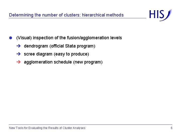
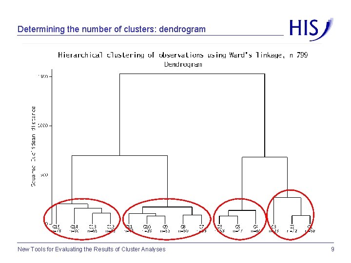
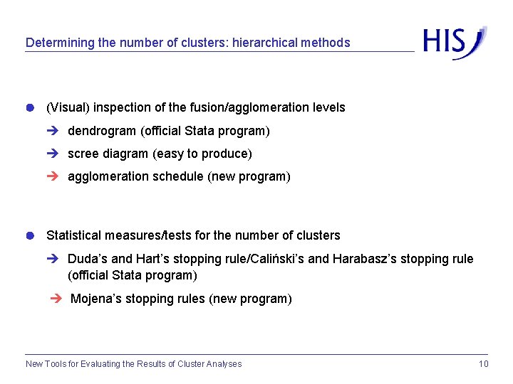
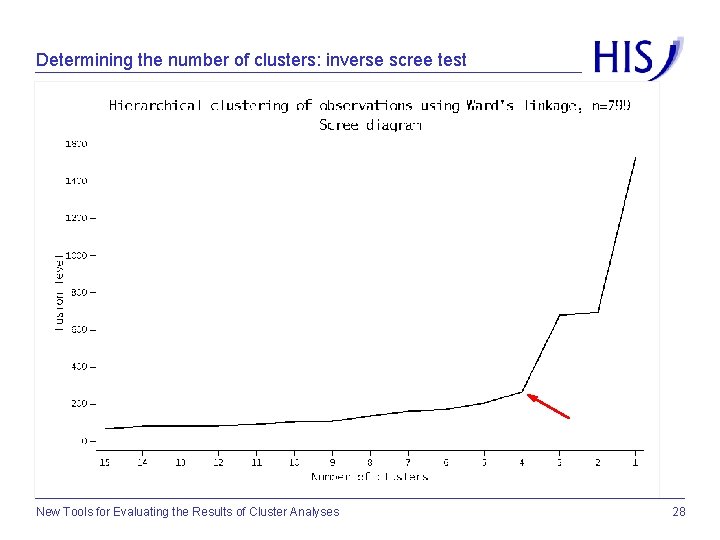
Determining the number of clusters: hierarchical methods (Visual) inspection of the fusion/agglomeration levels dendrogram (official Stata program) scree diagram (easy to produce) agglomeration schedule (new program) New Tools for Evaluating the Results of Cluster Analyses 6

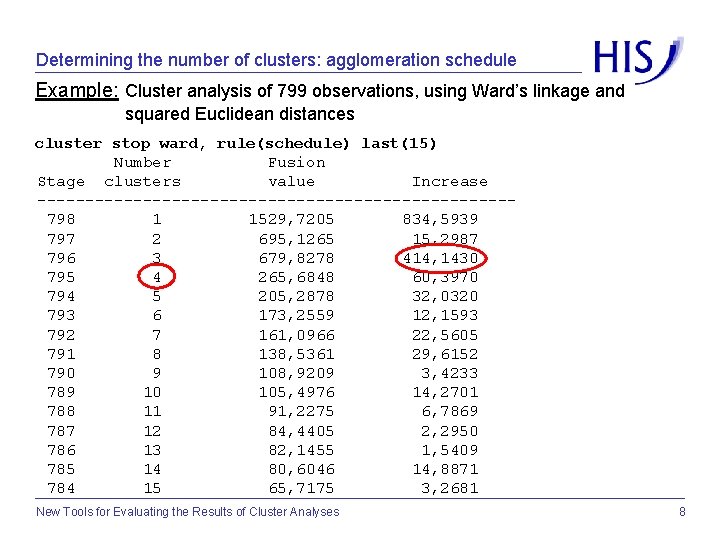
Determining the number of clusters: agglomeration schedule Syntax cluster stop [clname], rule(schedule) [laststeps(#)] Description cluster stop, rule(schedule) displays the agglomeration schedule for hierarchical agglomerative cluster analysis und computes the differences between the stages of the clustering process. Additional options laststeps(#) specifies the number of steps to be displayed. New Tools for Evaluating the Results of Cluster Analyses 7

Determining the number of clusters: agglomeration schedule Example: Cluster analysis of 799 observations, using Ward’s linkage and squared Euclidean distances cluster stop ward, rule(schedule) last(15) Number Fusion Stage clusters value Increase -------------------------798 1 1529, 7205 834, 5939 797 2 695, 1265 15, 2987 796 3 679, 8278 414, 1430 795 4 265, 6848 60, 3970 794 5 205, 2878 32, 0320 793 6 173, 2559 12, 1593 792 7 161, 0966 22, 5605 791 8 138, 5361 29, 6152 790 9 108, 9209 3, 4233 789 10 105, 4976 14, 2701 788 11 91, 2275 6, 7869 787 12 84, 4405 2, 2950 786 13 82, 1455 1, 5409 785 14 80, 6046 14, 8871 784 15 65, 7175 3, 2681 New Tools for Evaluating the Results of Cluster Analyses 8

Determining the number of clusters: dendrogram New Tools for Evaluating the Results of Cluster Analyses 9

Determining the number of clusters: hierarchical methods (Visual) inspection of the fusion/agglomeration levels dendrogram (official Stata program) scree diagram (easy to produce) agglomeration schedule (new program) Statistical measures/tests for the number of clusters Duda’s and Hart’s stopping rule/Caliński’s and Harabasz’s stopping rule (official Stata program) Mojena’s stopping rules (new program) New Tools for Evaluating the Results of Cluster Analyses 10

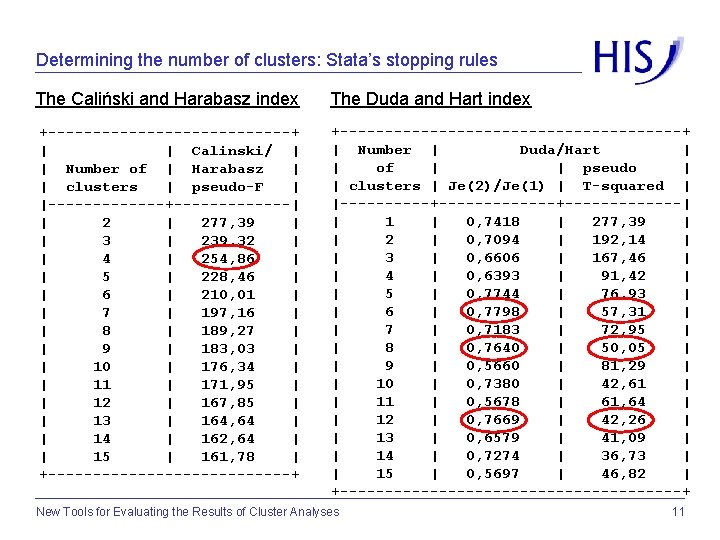
Determining the number of clusters: Stata’s stopping rules The Caliński and Harabasz index The Duda and Hart index +-------------------+ | Number | Duda/Hart | | of | pseudo | | clusters | Je(2)/Je(1) | T-squared | |----------+--------| | 1 | 0, 7418 | 277, 39 | | 2 | 0, 7094 | 192, 14 | | 3 | 0, 6606 | 167, 46 | | 4 | 0, 6393 | 91, 42 | | 5 | 0, 7744 | 76, 93 | | 6 | 0, 7798 | 57, 31 | | 7 | 0, 7183 | 72, 95 | | 8 | 0, 7640 | 50, 05 | | 9 | 0, 5660 | 81, 29 | | 10 | 0, 7380 | 42, 61 | | 11 | 0, 5678 | 61, 64 | | 12 | 0, 7669 | 42, 26 | | 13 | 0, 6579 | 41, 09 | | 14 | 0, 7274 | 36, 73 | | 15 | 0, 5697 | 46, 82 | +-------------------+ New Tools for Evaluating the Results of Cluster Analyses 11 +--------------+ | | Calinski/ | | Number of | Harabasz | | clusters | pseudo-F | |-------+-------| | 2 | 277, 39 | | 3 | 239, 32 | | 4 | 254, 86 | | 5 | 228, 46 | | 6 | 210, 01 | | 7 | 197, 16 | | 8 | 189, 27 | | 9 | 183, 03 | | 10 | 176, 34 | | 11 | 171, 95 | | 12 | 167, 85 | | 13 | 164, 64 | | 14 | 162, 64 | | 15 | 161, 78 | +--------------+

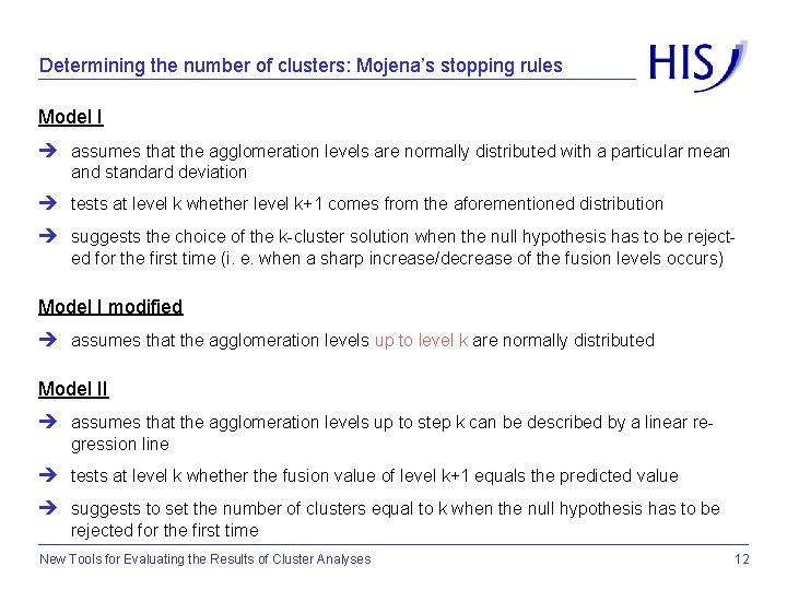
Determining the number of clusters: Mojena’s stopping rules Model I assumes that the agglomeration levels are normally distributed with a particular mean and standard deviation tests at level k whether level k+1 comes from the aforementioned distribution suggests the choice of the k-cluster solution when the null hypothesis has to be rejected for the first time (i. e. when a sharp increase/decrease of the fusion levels occurs) Model I modified assumes that the agglomeration levels up to level k are normally distributed Model II assumes that the agglomeration levels up to step k can be described by a linear regression line tests at level k whether the fusion value of level k+1 equals the predicted value suggests to set the number of clusters equal to k when the null hypothesis has to be rejected for the first time New Tools for Evaluating the Results of Cluster Analyses 12

Determining the number of clusters: Mojena’s stopping rules Syntax cluster stop [clname], rule(mojena) [laststeps(#) m 1 only] Description cluster stop, rule(mojena) calculates Mojena’s test statistics (Mojena I, Mojena I modified, and Mojena II) for determining the number of clusters of hierarchical agglomerative clustering methods and the corresponding significance levels. Additional options laststeps(#) specifies the number of steps to be displayed. m 1 only is used to suppress the calculation of Mojena I modified and Mojena II. New Tools for Evaluating the Results of Cluster Analyses 13

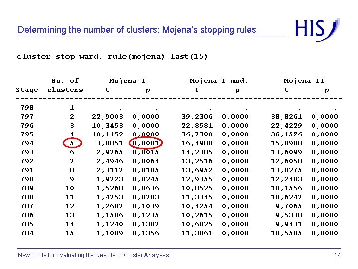
Determining the number of clusters: Mojena’s stopping rules cluster stop ward, rule(mojena) last(15) No. of Mojena I mod. Mojena II Stage clusters t p ------------------------------------ 798 1 . 797 2 22, 9003 0, 0000 39, 2306 0, 0000 38, 8261 0, 0000 796 3 10, 3453 0, 0000 22, 8581 0, 0000 22, 4229 0, 0000 795 4 10, 1152 0, 0000 36, 7300 0, 0000 36, 1526 0, 0000 794 5 3, 8851 0, 0001 16, 4988 0, 0000 15, 8908 0, 0000 793 6 2, 9765 0, 0015 14, 2385 0, 0000 13, 6099 0, 0000 792 7 2, 4946 0, 0064 13, 2516 0, 0000 12, 6058 0, 0000 791 8 2, 3117 0, 0105 13, 6952 0, 0000 13, 0275 0, 0000 790 9 1, 9723 0, 0245 12, 9355 0, 0000 12, 2483 0, 0000 789 10 1, 5268 0, 0636 10, 8525 0, 0000 10, 1556 0, 0000 788 11 1, 4753 0, 0703 11, 3345 0, 0000 10, 6247 0, 0000 787 12 1, 2607 0, 1039 10, 4254 0, 0000 9, 7065 0, 0000 786 13 1, 1586 0, 1235 10, 2615 0, 0000 9, 5338 0, 0000 785 14 1, 1240 0, 1307 10, 6825 0, 0000 9, 9431 0, 0000 784 15 1, 1009 0, 1356 11, 3061 0, 0000 10, 5505 0, 0000 New Tools for Evaluating the Results of Cluster Analyses 14

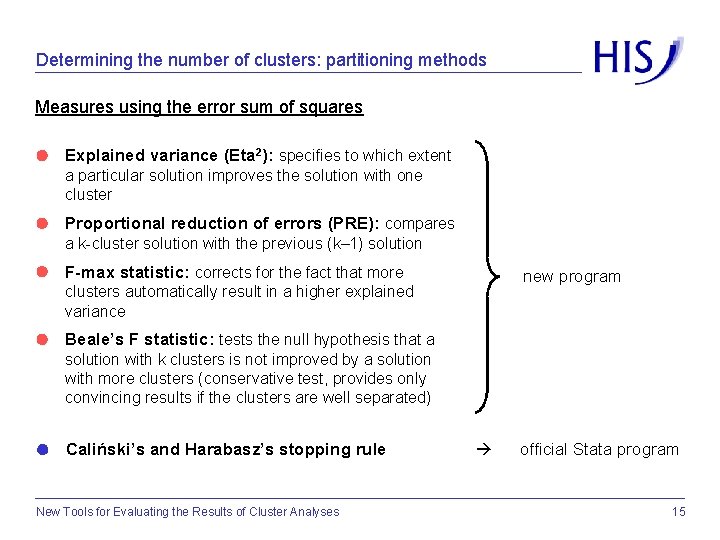
Determining the number of clusters: partitioning methods Measures using the error sum of squares Explained variance (Eta 2): specifies to which extent a particular solution improves the solution with one cluster Proportional reduction of errors (PRE): compares a k-cluster solution with the previous (k– 1) solution F-max statistic: corrects for the fact that more new program clusters automatically result in a higher explained variance Beale’s F statistic: tests the null hypothesis that a solution with k clusters is not improved by a solution with more clusters (conservative test, provides only convincing results if the clusters are well separated) Caliński’s and Harabasz’s stopping rule New Tools for Evaluating the Results of Cluster Analyses official Stata program 15

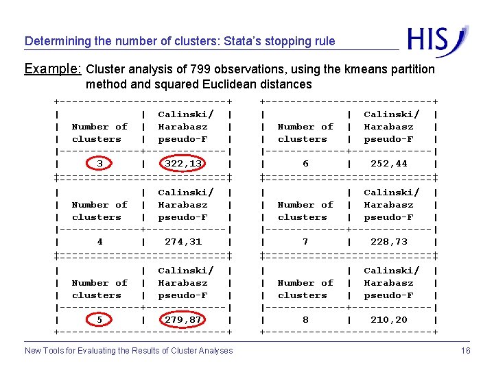
Determining the number of clusters: Stata’s stopping rule Example: Cluster analysis of 799 observations, using the kmeans partition method and squared Euclidean distances +--------------+ | | Calinski/ | | Number of | Harabasz | | clusters | pseudo-F | |-------+-------| | 3 | 322, 13 | +---------------------------+ +--------------+ | | Calinski/ | | Number of | Harabasz | | clusters | pseudo-F | |-------+-------| | 6 | 252, 44 | +---------------------------+ | | Calinski/ | | Number of | Harabasz | | clusters | pseudo-F | |-------+-------| | 4 | 274, 31 | +---------------------------+ | | Calinski/ | | Number of | Harabasz | | clusters | pseudo-F | |-------+-------| | 7 | 228, 73 | +---------------------------+ | | Calinski/ | | Number of | Harabasz | | clusters | pseudo-F | |-------+-------| | 5 | 279, 87 | +--------------+ | | Calinski/ | | Number of | Harabasz | | clusters | pseudo-F | |-------+-------| | 8 | 210, 20 | +--------------+ New Tools for Evaluating the Results of Cluster Analyses 16

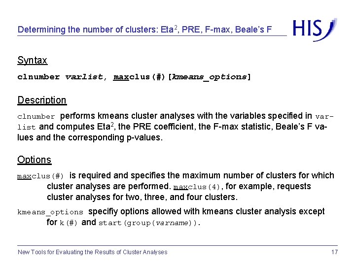
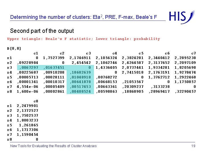
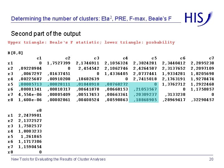
Determining the number of clusters: Eta 2, PRE, F-max, Beale’s F Syntax clnumber varlist, maxclus(#)[kmeans_options] Description clnumber performs kmeans cluster analyses with the variables specified in varlist and computes Eta 2, the PRE coefficient, the F-max statistic, Beale’s F va- lues and the corresponding p-values. Options maxclus(#) is required and specifies the maximum number of clusters for which cluster analyses are performed. maxclus(4), for example, requests cluster analyses for two, three, and four clusters. kmeans_options specifiy options allowed with kmeans cluster analysis except for k(#) and start(group(varname)). New Tools for Evaluating the Results of Cluster Analyses 17

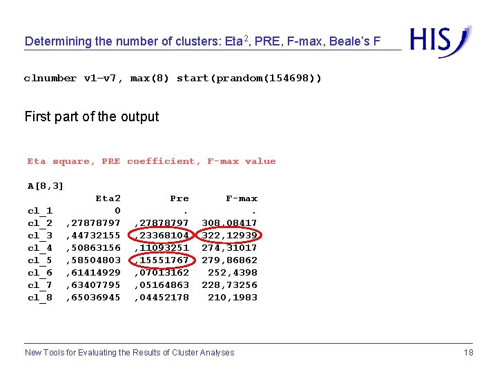
Determining the number of clusters: Eta 2, PRE, F-max, Beale’s F clnumber v 1–v 7, max(8) start(prandom(154698)) First part of the output Eta square, PRE coefficient, F-max value A[8, 3] Eta 2 Pre F-max cl_1 0 . cl_2 , 27878797 308, 08417 cl_3 , 44732155 , 23368104 322, 12939 cl_4 , 50863156 , 11093251 274, 31017 cl_5 , 58504803 , 15551767 279, 86862 cl_6 , 61414929 , 07013162 252, 4398 cl_7 , 63407795 , 05164863 228, 73256 cl_8 , 65036945 , 04452178 210, 1983 New Tools for Evaluating the Results of Cluster Analyses 18

Determining the number of clusters: Eta 2, PRE, F-max, Beale’s F Second part of the output Upper triangle: Beale‘s F statistic; lower triangle: probability B[8, 8] c 1 c 2 c 3 c 4 c 5 c 6 c 7 r 1 0 1, 7527399 2, 1746911 2, 1056324 2, 3824281 2, 3440412 2, 2895238 r 2 , 09228984 0 2, 454542 2, 1062746 2, 4264587 2, 3137652 2, 2097109 r 3 , 0067297 , 01637451 0 1, 4336405 2, 0737441 1, 9334281 1, 8205698 r 4 , 00225687 , 00910208 , 18682639 0 2, 7415018 2, 1763191 1, 9278474 r 5 , 00005713 , 00028111 , 01048918 , 00768272 0 1, 3762712 1, 2922468 r 6 , 00001341 , 00010317 , 00641878 , 00668153 , 21053567 0 1, 1750857 r 7 4, 554 e-06 , 00005409 , 00517453 , 00663361 , 20309237 , 3133238 0 r 8 1, 600 e-06 , 00002861 , 00408524 , 00598863 , 18868905 , 28969417 , 32290457 c 8 r 1 2, 2479901 r 2 2, 1372527 r 3 1, 7502537 r 4 1, 8003233 r 5 1, 261865 r 6 1, 1717306 r 7 1, 1590454 r 8 0 New Tools for Evaluating the Results of Cluster Analyses 19

Determining the number of clusters: Eta 2, PRE, F-max, Beale’s F Second part of the output Upper triangle: Beale‘s F statistic; lower triangle: probability B[8, 8] c 1 c 2 c 3 c 4 c 5 c 6 c 7 r 1 0 1, 7527399 2, 1746911 2, 1056324 2, 3824281 2, 3440412 2, 2895238 r 2 , 09228984 0 2, 454542 2, 1062746 2, 4264587 2, 3137652 2, 2097109 r 3 , 0067297 , 01637451 0 1, 4336405 2, 0737441 1, 9334281 1, 8205698 r 4 , 00225687 , 00910208 , 18682639 0 2, 7415018 2, 1763191 1, 9278474 r 5 , 00005713 , 00028111 , 01048918 , 00768272 0 1, 3762712 1, 2922468 r 6 , 00001341 , 00010317 , 00641878 , 00668153 , 21053567 0 1, 1750857 r 7 4, 554 e-06 , 00005409 , 00517453 , 00663361 , 20309237 , 3133238 0 r 8 1, 600 e-06 , 00002861 , 00408524 , 00598863 , 18868905 , 28969417 , 32290457 c 8 r 1 2, 2479901 r 2 2, 1372527 r 3 1, 7502537 r 4 1, 8003233 r 5 1, 261865 r 6 1, 1717306 r 7 1, 1590454 r 8 0 New Tools for Evaluating the Results of Cluster Analyses 20

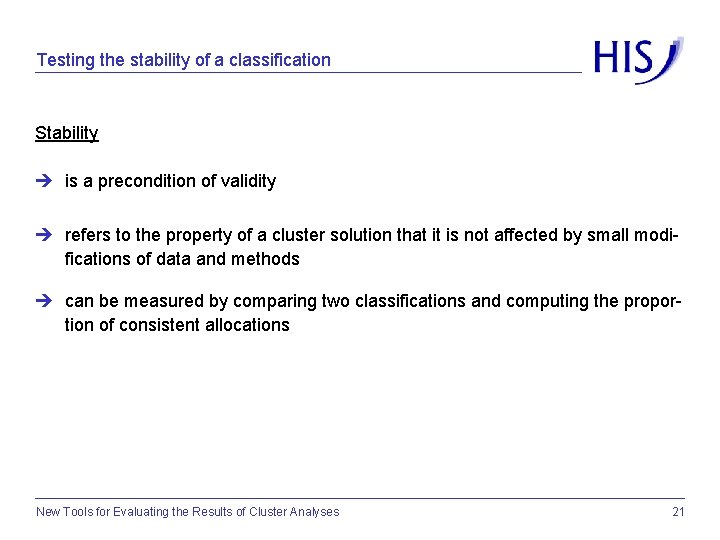
Testing the stability of a classification Stability is a precondition of validity refers to the property of a cluster solution that it is not affected by small modifications of data and methods can be measured by comparing two classifications and computing the proportion of consistent allocations New Tools for Evaluating the Results of Cluster Analyses 21

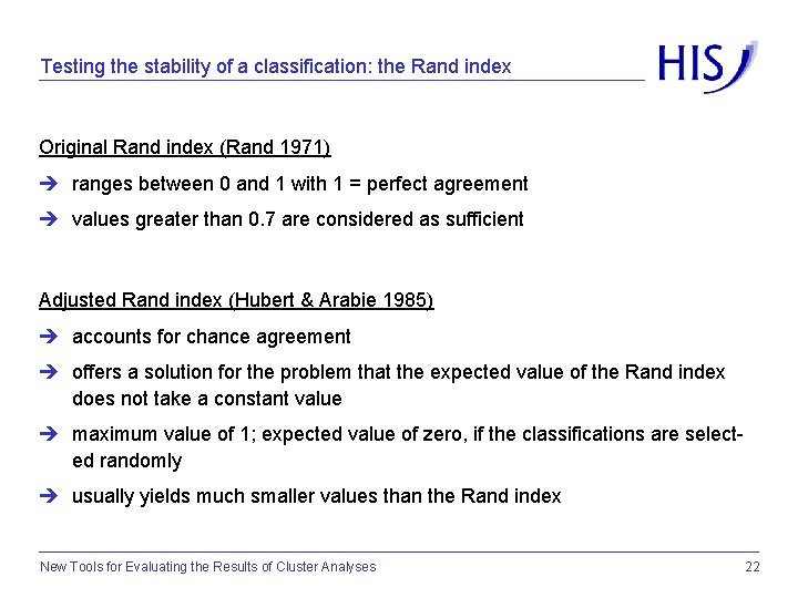
Testing the stability of a classification: the Rand index Original Rand index (Rand 1971) ranges between 0 and 1 with 1 = perfect agreement values greater than 0. 7 are considered as sufficient Adjusted Rand index (Hubert & Arabie 1985) accounts for chance agreement offers a solution for the problem that the expected value of the Rand index does not take a constant value maximum value of 1; expected value of zero, if the classifications are selected randomly usually yields much smaller values than the Rand index New Tools for Evaluating the Results of Cluster Analyses 22

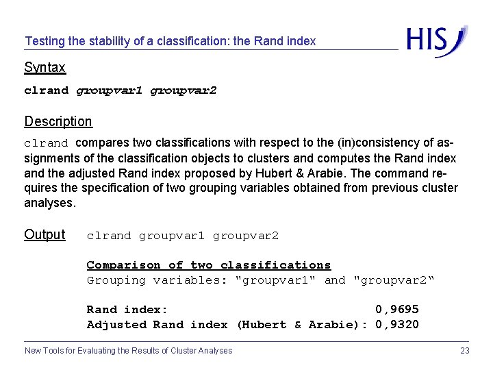
Testing the stability of a classification: the Rand index Syntax clrand groupvar 1 groupvar 2 Description clrand compares two classifications with respect to the (in)consistency of assignments of the classification objects to clusters and computes the Rand index and the adjusted Rand index proposed by Hubert & Arabie. The command requires the specification of two grouping variables obtained from previous cluster analyses. Output clrand groupvar 1 groupvar 2 Comparison of two classifications Grouping variables: "groupvar 1" and "groupvar 2“ Rand index: 0, 9695 Adjusted Rand index (Hubert & Arabie): 0, 9320 New Tools for Evaluating the Results of Cluster Analyses 23

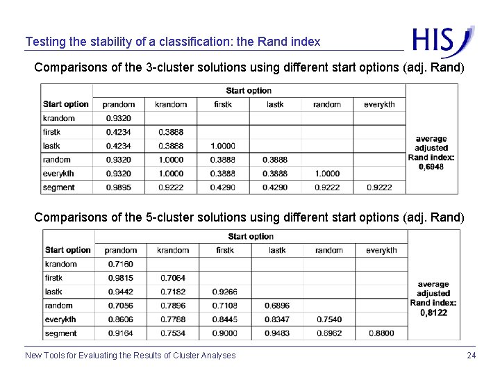
Testing the stability of a classification: the Rand index Comparisons of the 3 -cluster solutions using different start options (adj. Rand) Comparisons of the 5 -cluster solutions using different start options (adj. Rand) New Tools for Evaluating the Results of Cluster Analyses 24

Outlook speeding up the program for calculating Mojena’s stopping rules improvement of clnumber improvement of clrand new program for checking whether a local minimum is found with kmeans or kmedians cluster analysis new programs for calculating additional statistics (e. g. homogeneity measures, measures for the fit of a dendrogram) New Tools for Evaluating the Results of Cluster Analyses 25

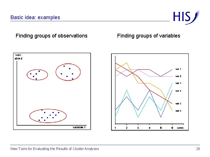
Basic idea: examples Finding groups of observations New Tools for Evaluating the Results of Cluster Analyses Finding groups of variables 26

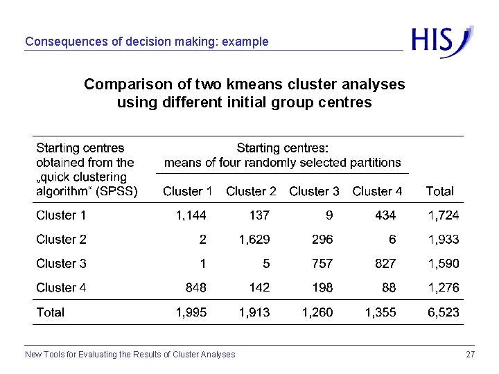
Consequences of decision making: example Comparison of two kmeans cluster analyses using different initial group centres New Tools for Evaluating the Results of Cluster Analyses 27

Determining the number of clusters: inverse scree test New Tools for Evaluating the Results of Cluster Analyses 28