Extending Stata graphics via SVG manipulation commands Robert

Extending Stata graphics via SVG manipulation commands

Robert Grant, Bayes. Camp Tim Morris, MRC Clinical Trials Unit at UCL

Stata 14’s best feature On upgrading Stata, one of the pieces of housekeeping I do is change stuff in graph set. Things like: . graph set print logo off On submitting ‘graph set’, I spotted something unfamiliar…

Stata 14’s best feature

Stata 14’s best feature

What is SVG?
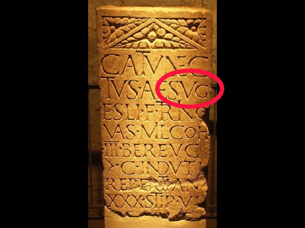

Raster graphics 119 KB. png

Vector graphics 12 KB. svg

Read it
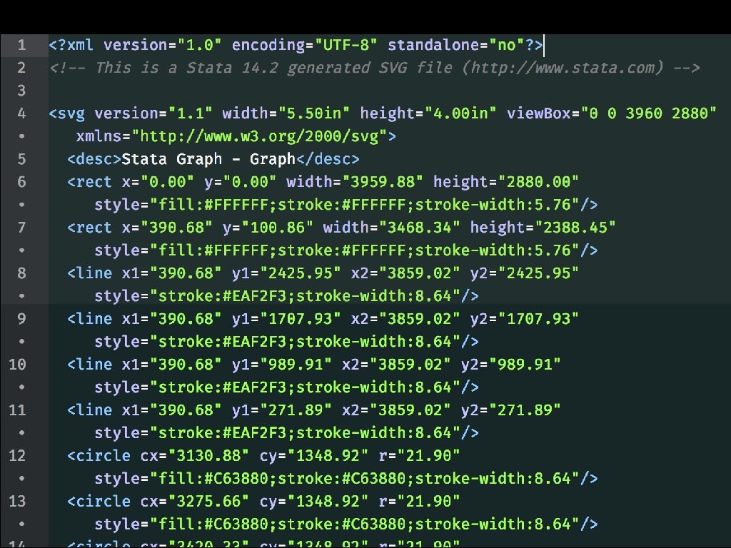

Build it
 • Open it")
General principle • Get an SVG file out of Stata (14+) • Open it up and make it even cooler • Receive the accolades of your peers

WIN!

SVG permits ‘opacity=#’

Semi-transparency • or semi-opacity, or translucency • Add to the style information of objects • stroke-opacity, fill-opacity, etc. • Job done!
 in Stata 15 Yes!")
Semi-transparency But Tim, I can just do this with mcol(%60) in Stata 15 Yes! …sort of
")
Translucency is easyish (filefilter)
")
Stata 15 made it so simple: mcol(%60)

Let me break it down By hand Stata 15 ‘%’ syntax

BUT… Stata. Corp? In Stata 14, a circle was written as: In Stata 15 a circle is now written as: This is a problem of general graphics rendering. mlalign(center) fixes it. (thx Chinh Nguyen)
 Translucency ‘by hand’ is reasonably easy (harder in Stata")
If you care (I do) Translucency ‘by hand’ is reasonably easy (harder in Stata 15 than in 14). tempfile a b. graph export `a' , as(svg). filefilter `a' `b', from(fill: none; stroke: #606060; ) > to(fill: none; stroke: none; ). filefilter `b' scatter-trans. svg, from(fill: #606060) > to(fill: #606060; fill-opacity: 0. 6) replace

Translucency for lines
, such as a map, in")
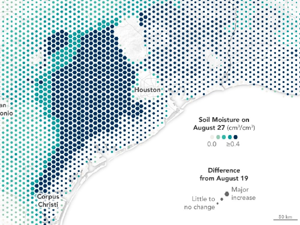
Semi-transparency • Now you can add an image (raster), such as a map, in the background
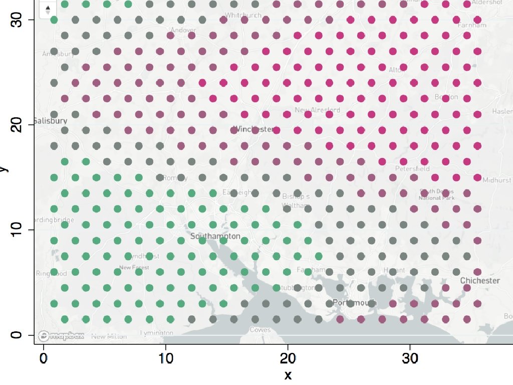


Hexagonal binning • This is different: we don’t start with a Stata SVG file • Count observations in hexagons • Make a scatterplot on a grid -> SVG • Open that and replace circles with hexagon symbols • Job done!
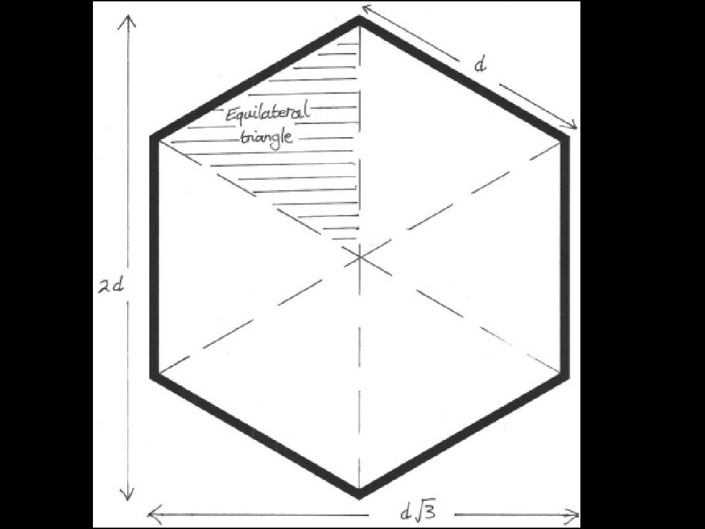
 • • We can set up the honeycomb: two grids")
Doing hexbin (0, 1) • • We can set up the honeycomb: two grids of rectangles with y and x offset (0. 5√ 3, 0. 5) (– 0. 5√ 3, 0. 5) (0, 0) Get binning! (– 0. 5√ 3, – 0. 5) (0, – 1)

Bivariate normal

Stata gets us this far

After editing SVG from Stata…

and with a background image

Interactivity • Add basic HTML before & after the SVG • Now you have a web page • Connect objects to controls like sliders, buttons, etc with Java. Script • Job done!

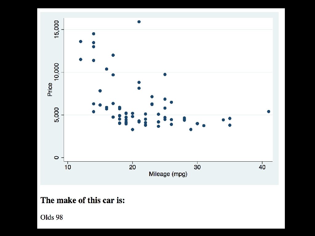
Interactivity • sysuse auto • scatter price mpg • graph export "example. svg", replace • svgwithjs "example. svg", htmlfile("output. html") movar(make) moheading("The make of this car is: ")
 • Animation (see Sarah Drasner) •")
and more… • Colour gradients (see Nadieh Bremer) • Animation (see Sarah Drasner) • What are your ideas?

Pre-emptive wishes & grumbles

Why not • Add id and class to objects • Get rid of the double markers in version 15! • Write out the SVG file without “drawing a graph”: SVG file becomes the graph window . graph gtype ->. svg gtype

Thanks for listening github. com/robertgrant/stata-svg
- Slides: 41