Exploratory Factor Analysis STA 431 Spring 2013 See

Exploratory Factor Analysis STA 431: Spring 2013 See last slide for copyright information

Factor Analysis: The Measurement Model D 1 D 2 D 3 F 1 D 4 D 5 D 7 D 6 F 2 D 8

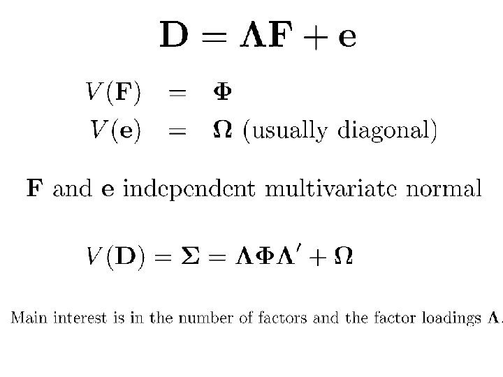
Example with 2 factors and 8 observed variables The lambda values are called factor loadings.

Terminology • The lambda values are called factor loadings. • F 1 and F 2 are sometimes called common factors, because they influence all the observed variables. • Error terms e 1, …, e 8 are sometimes called unique factors, because each one influences only a single observed variable.

Factor Analysis can be • Exploratory: The goal is to describe and summarize the data by explaining a large number of observed variables in terms of a smaller number of latent variables (factors). The factors are the reason the observable variables have the correlations they do. • Confirmatory: Statistical estimation and testing as usual.

Part One: Unconstrained (Exploratory) Factor Analysis

A Re-parameterization

Parameters are not identifiable • Two distinct (Lambda, Phi) pairs give the same Sigma, and hence the same distribution of the data. • Actually, there are infinitely many. Let Q be an arbitrary covariance matrix for F.

Parameters are not identifiable • This shows that the parameters of the general measurement model are not identifiable without some restrictions on the possible values of the parameter matrices. • Notice that the general unrestricted model could be very close to the truth. But the parameters cannot be estimated successfully, period.

Restrict the model • Set Phi = the identity, so V(F) = I • All the factors are standardized, as well as independent. • Justify this on the grounds of simplicity. • Say the factors are “orthogonal” (at right angles, uncorrelated).

Standardize the observed variables too • For j = 1, …, k and independently for i=1, …, n • • Assume each observed variable has variance one as well as mean zero. • Sigma is now a correlation matrix. • Base inference on the sample correlation matrix.

Revised Exploratory Factor Analysis Model

Meaning of the factor loadings • λij is the correlation between variable i and factor j. • Square of λij is the reliability of variable i as a measure of factor j.

Communality is the proportion of variance in variable i that comes from the common factors. • It is called the communality of variable i. • The communality cannot exceed one. • Peculiar? •

If we could estimate the factor loadings • We could estimate the correlation of each observable variable with each factor. • We could easily estimate reliabilities. • We could estimate how much of the variance in each observable variable comes from each factor. • This could reveal what the underlying factors are, and what they mean. • Number of common factors can be very important too.

Examples • A major study of how people describe objects (using 7 -point scales from Ugly to Beautiful, Strong to Weak, Fast to Slow etc. revealed 3 factors of connotative meaning: – Evaluation – Potency – Activity • Factor analysis of a large collection of personality scales revealed 2 major factors: – Neuroticism – Extraversion • Yet another study led to 16 personality factors, the basis of the widely used 16 pf test.

Rotation Matrices

The transpose rotated the axies back through an angle of minus theta.

In General • A pxp matrix R satisfying R-inverse = Rtranspose is called an orthogonal matrix. • Geometrically, pre-multiplication by an orthogonal matrix corresponds to a rotation in p-dimensional space. • If you think of a set of factors F as a set of axies (underlying dimensions), then RF is a rotation of the factors. • Call it an orthoganal rotation, because the factors remain uncorrelated (at right angles).

Another Source of non-identifiability Infinitely many rotation matrices produce the same Sigma.

New Model

A Solution • Place some restrictions on the factor loadings, so that the only rotation matrix that preserves the restrictions is the identity matrix. For example, λij = 0 for j>i • There are other sets of restrictions that work. • Generally, they result in a set of factor loadings that are impossible to interpret. Don’t worry about it. • Estimate the loadings by maximum likelihood. Other methods are possible but used much less than in the past. • All (orthoganal) rotations result in the same value of the likelihood function (the maximum is not unique). • Rotate the factors (that is, post-multiply the loadings by a rotation matrix) so as to achieve a simple pattern that is easy to interpret.

Rotate the factor solution • Rotate the factors to achieve a simple pattern that is easy to interpret. • There are various criteria. They are all iterative, taking a number of steps to approach some criterion. • The most popular rotation method is varimax rotation. • Varimax rotation tries to maximize the (squared) loading of each observable variable with just one underlying factor. • So typically each variable has a big loading on (correlation with) one of the factors, and small loadings on the rest. • Look at the loadings and decide what the factors mean (name the factors).

A Warning • When a non-statistician claims to have done a “factor analysis, ” ask what kind. • Usually it was a principal components analysis. • Principal components are linear combinations of the observed variables. They come from the observed variables by direct calculation. • In true factor analysis, it’s the observed variables that arise from the factors. • So principal components analysis is kind of like backwards factor analysis, though the spirit is similar. • Most factor analysis (SAS, SPSS, etc. ) does principal components analysis by default.

Copyright Information This slide show was prepared by Jerry Brunner, Department of Statistics, University of Toronto. It is licensed under a Creative Commons Attribution - Share. Alike 3. 0 Unported License. Use any part of it as you like and share the result freely. These Powerpoint slides are available from the course website: http: //www. utstat. toronto. edu/~brunner/oldclass/431 s 13