Introduction to Regression with Measurement Error STA 431

Introduction to Regression with Measurement Error STA 431: Spring 2015 See last slide for copyright information

Measurement Error Snack food consumption Exercise Income Cause of death Even amount of drug that reaches animal’s blood stream in an experimental study • Is there anything that is not measured with error? • • •

For categorical variables Classification error is common

Additive measurement error: W X e

Simple additive model for measurement error: Continuous case

How much of the variation in the observed variable comes from variation in the quantity of interest, and how much comes from random noise?

Reliability is the squared correlation between the observed variable and the latent variable (true score). First, recall

Reliability

Reliability is the proportion of the variance in the observed variable that comes from the latent variable of interest, and not from random error.

Correlate usual measurement with “Gold Standard? ” Not very realistic, except maybe for some bio-markers

Measure twice e 1 W 2 X e 2

Test-Retest Equivalent measurements

Test-Retest Reliability

Estimate the reliability: Measure twice for a sample of size n Calculate the sample correlation between W 1, 1 , W 2, 1 , …, Wn, 1 W 1, 2 , W 2, 2 , …, Wn, 2 • Test-retest reliability • Alternate forms reliability • Split-half reliability

The consequences of ignoring measurement error in the explanatory (x) variables First look at measurement error in the response variable

Measurement error in the response variable

Measurement error in the response variable is a less serious problem: Re-parameterize Can’t know everything, but all we care about is β 1 anyway.

Whenever a response variable appears to have no measurement error, assume it does have measurement error but the problem has been reparameterized.

Measurement error in the explanatory variables

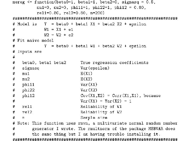
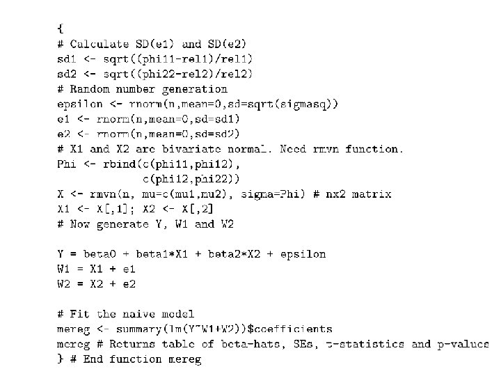
Measurement error in the explanatory variables • True model • Naïve model

True Model (More detail)

Reliabilities • Reliability of W 1 is • Reliability of W 2 is

Test X 2 controlling for (holding constant) X 1 That's the usual conditional model

Unconditional: Test X 2 controlling for X 1 Hold X 1 constant at fixed x 1

Controlling Type I Error Probability • Type I error is to reject H 0 when it is true, and there is actually no effect or no relationship • Type I error is very bad. Maybe that’s why it’s called an “error of the first kind. ” • False knowledge is worse than ignorance.

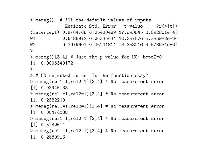
Simulation study: Use pseudorandom number generation to create data sets • • Simulate data from the true model with β 2=0 Fit naïve model Test H 0: β 2=0 at α = 0. 05 using naïve model Is H 0 rejected five percent of the time?

Try it with measurement error 9 out of 10

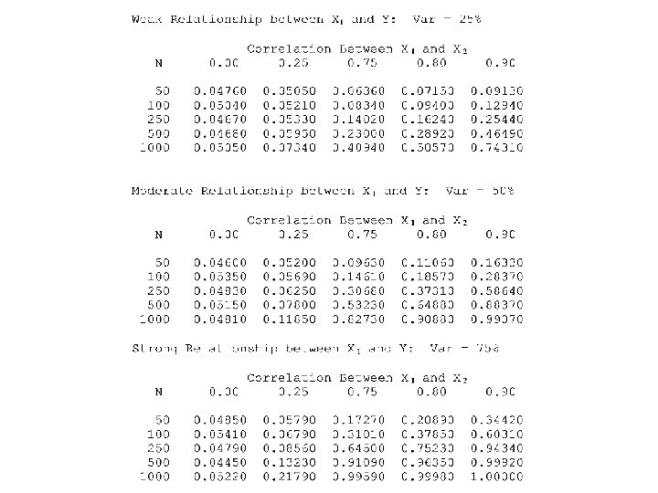
A Big Simulation Study (6 Factors) • • • Sample size: n = 50, 100, 250, 500, 1000 Corr(X 1, X 2): ϕ 12 = 0. 00, 0. 25, 0. 75, 0. 80, 0. 90 Variance in Y explained by X 1: 0. 25, 0. 50, 0. 75 Reliability of W 1: 0. 50, 0. 75, 0. 80, 0. 95 Reliability of W 2: 0. 50, 0. 75, 0. 80, 0. 95 Distribution of latent variables and error terms: Normal, Uniform, t, Pareto • 5 x 5 x 3 x 5 x 5 x 4 = 7, 500 treatment combinations

Within each of the • • 5 x 5 x 3 x 5 x 5 x 4 = 7, 500 treatment combinations 10, 000 random data sets were generated For a total of 75 million data sets All generated according to the true model, with β 2=0 • Fit naïve model, test H 0: β 2=0 at α = 0. 05 • Proportion of times H 0 is rejected is a Monte Carlo estimate of the Type I Error Probability

Look at a small part of the results • Both reliabilities = 0. 90 • Everything is normally distributed • β 0 = 1, β 1=1, β 2=0 (H 0 is true)

Marginal Mean Type I Error Probabilities

Summary • Ignoring measurement error in the independent variables can seriously inflate Type I error probabilitys. • The poison combination is measurement error in the variable for which you are “controlling, ” and correlation between latent independent variables. If either is zero, there is no problem. • Factors affecting severity of the problem are (next slide)

Factors affecting severity of the problem • As the correlation between X 1 and X 2 increases, the problem gets worse. • As the correlation between X 1 and Y increases, the problem gets worse. • As the amount of measurement error in X 1 increases, the problem gets worse. • As the amount of measurement error in X 2 increases, the problem gets less severe. • As the sample size increases, the problem gets worse. • Distribution of the variables does not matter much.

As the sample size increases, the problem gets worse. For a large enough sample size, no amount of measurement error in the independent variables is safe, assuming that the latent independent variables are correlated.

The problem applies to other kinds of regression, and various kinds of measurement error • Logistic regression • Proportional hazards regression in survival analysis • Log-linear models: Test of conditional independence in the presence of classification error • Median splits • Even converting X 1 to ranks inflates Type I Error probability

If X 1 is randomly assigned • Then it is independent of X 2: Zero correlation. • So even if an experimentally manipulated variable is measured (implemented) with error, there will be no inflation of Type I error probability. • If X 2 is randomly assigned and X 1 is a covariate observed with error (very common), then again there is no correlation between X 1 and X 2, and so no inflation of Type I error probability. • Measurement error may decrease the precision of experimental studies, but in terms of Type I error it creates no problems. • This is good news!

What is going on theoretically? First, need to look at some largesample tools

Sample Space Ω, ω an element of Ω • Observing whether a single individual is male or female: • Pair of individuals and observed their genders in order: • Select n people and count the number of females: • For limits problems, the points in Ω are infinite sequences

Random variables are functions from Ω into the set of real numbers

Random sample To see what happens for large samples

Modes of Convergence • Almost Sure Convergence • Convergence in Probability • Convergence in Distribution

Almost Sure Convergence Acts like an ordinary limit, except possibly on a set of probability zero. All the usual rules apply.

Strong Law of Large Numbers The only condition required for this to hold is the existence of the expected value.

Let X 1, …, Xn be independent and identically distributed random variables; let X be a general random variable from this same distribution, and Y=g(X)

So for example That is, sample moments converge almost surely to population moments.

Convergence in Probability Almost Sure Convergence => Convergence in Probability Strong Law of Large Numbers => Weak Law of Large Numbers

Convergence in Distribution Central Limit Theorem says

Connections among the Modes of Convergence

Consistency Tn = Tn(X 1, …, Xn) is a statistic estimating a parameter θ Strong consistency implies ordinary consistency.

Consistency is great but it's not enough • It means that as the sample size becomes indefinitely large, you (probably) get as close as you like to the truth. • It's the least we can ask. Estimators that are not consistent are completely unacceptable for most purposes.

Consistency of the Sample Variance

Consistency of the Sample Covariance

MOM is consistent, usually

True Regression model: Single explanatory variable measured with error

Single Explanatory Variable • True model • Naive model

Least squares estimate of β 1 for the Naïve Model

• Goes to the true parameter times reliability of W. • Asymptotically biased toward zero, because reliability is between zero and one. • No asymptotic bias when β 1=0. • No inflation of Type I error probability • Loss of power when β 1 ≠ 0 • Measurement error just makes relationship seem weaker than it is. Reassuring, but watch out!

Two explanatory variables with error

Two explanatory variables, β 2=0

Least squares estimate of β 2 for the Naïve Model when true β 2 = 0 Combined with estimated standard error going almost surely to zero, Get t statistic for H 0: β 2 = 0 going to ±∞, and p-value going almost Surely to zero, unless. .

Combined with estimated standard error going almost surely to zero, get t statistic for H 0: β 2 = 0 going to ±∞, and p-value going almost surely to zero, unless. . • There is no measurement error in W 1, or • There is no relationship between X 1 and Y, or • There is no correlation between X 1 and X 2. And, anything that increases Var(W 2) will make the problem less severe.

Need a statistical model that includes measurement error

Copyright Information This slide show was prepared by Jerry Brunner, Department of Statistics, University of Toronto. It is licensed under a Creative Commons Attribution - Share. Alike 3. 0 Unported License. Use any part of it as you like and share the result freely. These Powerpoint slides are available from the course website: http: //www. utstat. toronto. edu/~brunner/oldclass/431 s 15