Structural Equation Models The General Case STA 431

Structural Equation Models: The General Case STA 431: Spring 2015 See last slide for copyright information

An Extension of Multiple Regression • More than one regression-like equation • Includes latent variables • Variables can be explanatory in one equation and response in another • Modest changes in notation • Vocabulary • Path diagrams • No intercepts, all expected values zero • Serious modeling (compared to ordinary statistical models) • Parameter identifiability

Variables can be response in one equation and explanatory in another • Variables (IQ = Intelligence Quotient): – X 1 = Mother’s adult IQ – X 2 = Father’s adult IQ – Y 1 = Person’s adult IQ – Y 2 = Child’s IQ in Grade 8 • Of course all these variables are measured with error. • We will lose the intercepts very soon.

Modest changes in notation • Regression coefficients are now called gamma instead of beta • Betas are used for links between Y variables • Intercepts are alphas but they will soon disappear. • We feel free to drop the subscript i; implicitly, everything is independent and identically distributed for i = 1, …, n.

Vocabulary • Variables can be Latent or Manifest. – Manifest means observable – All error terms are latent • Variables can be Exogenous or Endogenous – Exogenous variables appear only on the right side of the = sign. • Think “X” for explanatory variable. • All error terms are exogenous – Endogenous variables appear on the left of at least one = sign. • Think “end” of an arrow pointing from exogenous to endogenous • Betas link endogenous variables to other endogenous variables.

Path diagrams

Path Diagram Rules • Latent variables are enclosed by ovals. • Observable (manifest) variables are enclosed by rectangles. • Error terms are not enclosed – Sometimes the arrows from the error terms seem to come from nowhere. The symbol for the error term does not appear in the path diagram. – Sometimes there are no arrows for the error terms at all. It is just assumed that such an arrow points to each endogenous variable. • Straight, single-headed arrows point from each variable on the right side of an equation to the endogenous variable on the left side. – Sometimes the coefficient is written on the arrow, but sometimes it is not. • A curved, double-headed arrow between two variables (always exogenous variables) means they have a non-zero covariance. – Sometimes the symbol for the covariance is written on the curved arrow, but sometimes it is not.

Causal Modeling (cause and effect) • The arrows deliberately imply that if A B, we are saying A contributes to B, or partly causes it. • There may be other contributing variables. All the ones that are unknown are lumped together in the error term. • Are these unknown variables are independent of the variables in the model? Probably not. • Sometimes we can get around the problem with instrumental variables.

Serious Modeling • Once you accept that model equations are statements about what contributes to what, you realize that structural equation models represent a rough theory of the data, with some parts (the parameter values) unknown. • They are somewhere between ordinary statistical models, which are like one-size-fits-all clothing, and true scientific models, which are like tailor made clothing. • So they are very flexible and potentially valuable. It is good to combine what the data can tell you with what you already know. • But structural equation models can require a lot of input and careful thought to construct. In this course, we will get by mostly on common sense. • In general, the parameters of the most reasonable model need not be identifiable. It depends upon the form of the data as well as on the model. Identifiability needs to be checked. Frequently, this can be done by inspection.

Example: Halo Effects in Real Estate

Losing the intercepts and expected values • Mostly, the intercepts and expected values are not identifiable anyway, as in multiple regression with measurement error. • We have a chance to identify a function of the parameter vector – the parameters that appear in the covariance matrix Σ = V(D). • Re-parameterize. The new parameter vector is the set of parameters in Σ, and also μ = E(D). Estimate μ with x -bar, forget it, and concentrate on inference for the parameters in Σ. • To make calculation of the covariance matrix easier, write the model equations in centered form. The little letters c over the variables are invisible.

From this point on the models have no means and no intercepts. Now more examples

Multiple Regression X 1 Y X 2

Regression with measurement error

A Path Model with Measurement Error

A Factor Analysis Model e 1 e 2 e 3 e 4 e 5 X 1 X 2 X 3 X 4 X 5 General Intelligence

A Longitudinal Model M 1 M 2 M 3 M 4 P 1 P 2 P 3 P 4

Estimation and Testing as Before X Y 1 Y 2

Distribution of the data

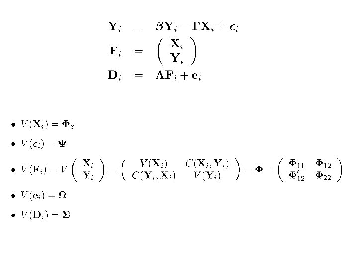
A General Two-Stage Model

More Details

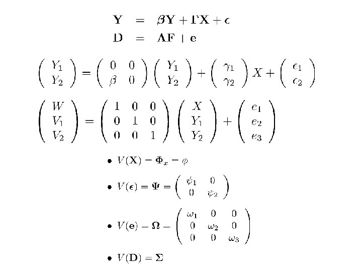
Recall the example

Observable variables in the latent variable model (fairly common) • These present no problem • Let P(ej=0) = 1, so Var(ej) = 0 • And Cov(ei, ej)=0 because if P(ej=0) = 1 • So in the covariance matrix Ω=V(e), just set ωij = ωji = 0, i=1, …, k

What should you be able to do? • Given a path diagram, write the model equations and say which exogenous variables are correlated with each other. • Given the model equations and information about which exogenous variables are correlated with each other, draw the path diagram. • Given either piece of information, write the model in matrix form and say what all the matrices are. • Calculate model covariance matrices • Check identifiability

Recall the notation

For the latent variable model, calculate Φ = V(F) So,

For the measurement model, calculate Σ = V(D)

Two-stage Proofs of Identifiability • Show the parameters of the measurement model (Λ, Φ, Ω) can be recovered from Σ= V(D). • Show the parameters of the latent variable model (β, Γ, Φ 11, Ψ) can be recovered from Φ = V(F). • This means all the parameters can be recovered from Σ. • Break a big problem into two smaller ones. • Develop rules for checking identifiability at each stage.

Copyright Information This slide show was prepared by Jerry Brunner, Department of Statistics, University of Toronto. It is licensed under a Creative Commons Attribution - Share. Alike 3. 0 Unported License. Use any part of it as you like and share the result freely. These Powerpoint slides are available from the course website: http: //www. utstat. toronto. edu/~brunner/oldclass/431 s 15