Epipolar lines epipolar plane epipolar lines O Baseline

Epipolar lines epipolar plane epipolar lines O Baseline O’

Rectification • Rectification: rotation and scaling of each camera’s coordinate frame to make the epipolar lines horizontal and equi-height, by bringing the two image planes to be parallel to the baseline • Rectification is achieved by applying homography to each of the two images

Rectification O Baseline O’

Cyclopean coordinates •

Disparity •

Random dot stereogram • Depth can be perceived from a random dot pair of images (Julesz) • Stereo perception is based solely on local information (low level)

Moving random dots

Compared elements •

Dynamic programming • Each pair of epipolar lines is compared independently • Local cost, sum of unary term and binary term – Unary term: cost of a single match – Binary term: cost of change of disparity (occlusion) • Analogous to string matching (‘diff’ in Unix)

String matching • Swing → String S Start t r i n g S w i n g End

String matching • Cost: #substitutions + #insertions + #deletions S t r i n g S w i n g
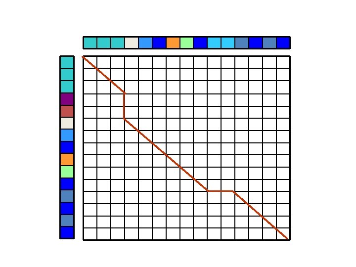

Dynamic Programming • Shortest path in a grid • Diagonals: constant disparity • Moving along the diagonal – pay unary cost (cost of pixel match) • Move sideways – pay binary cost, i. e. disparity change (occlusion, right or left) • Cost prefers fronto-parallel planes. Penalty is paid for tilted planes

Dynamic Programming Start

Probability interpretation: Viterbi algorithm •

Markov Random Field •
 •")
Iterated Conditional Modes (ICM) •

Graph cuts: expansion moves •

α-Expansion •
")
α-Expansion (1 D example)
")
α-Expansion (1 D example)
")
α-Expansion (1 D example)
")
α-Expansion (1 D example)
")
α-Expansion (1 D example)
")
α-Expansion (1 D example)
")
α-Expansion (1 D example)
")
α-Expansion (1 D example)
")
α-Expansion (1 D example)

Common Metrics •

Reconstruction with graph-cuts Original Result Ground truth
- Slides: 30