Geometry 2 Epipolar Lines Introduction to Computer Vision

Geometry 2: Epipolar Lines Introduction to Computer Vision Ronen Basri Weizmann Institute of Science

Material covered • Pinhole camera model, perspective projection • A taste of projective geometry • Homography (planes, camera rotation) • Two view geometry, general case: • Epipolar geometry, the essential matrix • Camera calibration, the fundamental matrix • Stereo vision • 3 D reconstruction from two views • Multi-view geometry, reconstruction through factorization

Hierarchy of transformations Rigid Preserves angles, lengths, area, parallelism Similarity Preserves angles, parallelism Affine Preserves parallelism Homography Preserves cross ratio

Camera rotation •

Planar scene •

Camera matrix •

Calibration matrix •

Two view geometry epipolar line

Epipolar plane Definition: Epipolar plane: a plane that contains the baseline epipolar plane Baseline epipolar line

Epipoles • • • Each epipolar plane produces a pair of epipolar lines There is a 1 -D system of epipolar planes All epipolar planes contain the baseline All epipolar lines intersect at the epipole An epipole is the projection of the right focal center onto the left image (and vice versa) epipolar lines Baseline

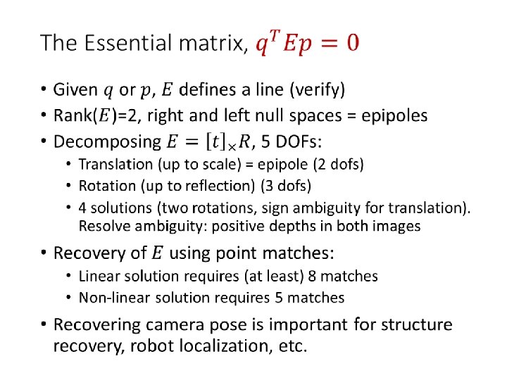
Epipolar constraints: the essential matrix • Epipolar plane Baseline

Cross product, triple product •

Epipolar constraints: the Essential matrix •

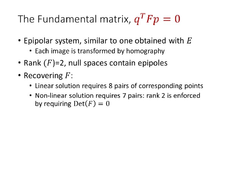
Uncalibrated case: the Fundamental matrix •

Summary Homography Perspective (calibrated) Perspective (uncalibrated) Orthographic One-to-one (group) Concentric epipolar lines Parallel epipolar lines Form Properties DOFs 8(5) 8(7) 4 Eqs/pnt 2 1 1 1 Minimal configuration 4 5+ (8, linear) 7+ (8, linear) 4 Depth No Yes, up to scale Yes, projective Affine structure (third view required for Euclidean structure)

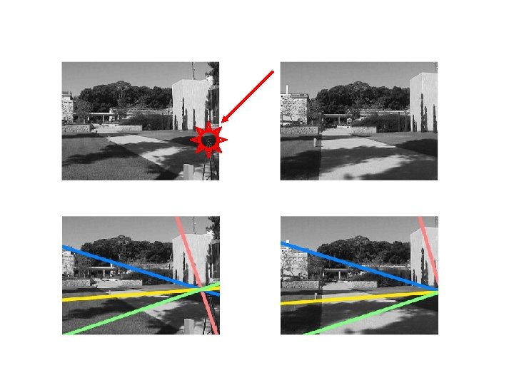
Recovering epipolar constraints

Recovering epipolar constraints: pipeline •

SIFT matches

Epipolar lines

Rectification • Homography to make epipolar lines horizontal Baseline O O’

Rectification Baseline O O’

Disparity •

The correspondence problem • Stereo matching is ill-posed: • Matching ambiguity: different regions may look similar

The correspondence problem • Stereo matching is ill-posed: • Matching ambiguity: different regions may look similar • Specular reflectance: multiple depth values

Random dot stereogram • Depth is perceived from a pair of random dot images • Stereo perception is based solely on local information (low level)

Moving random dots

Dynamic programming • Each pair of epipolar lines is compared independently • Local cost, sum of unary term and binary term • Unary term: cost of a single match • Binary term: cost of change of disparity (occlusion) • Analogous to string matching (‘diff’ in Unix)

String matching • Swing → String S t r i n g Start S w i n g End

String matching • Cost: #substitutions + #insertions + #deletions S t r i n g S w i n g

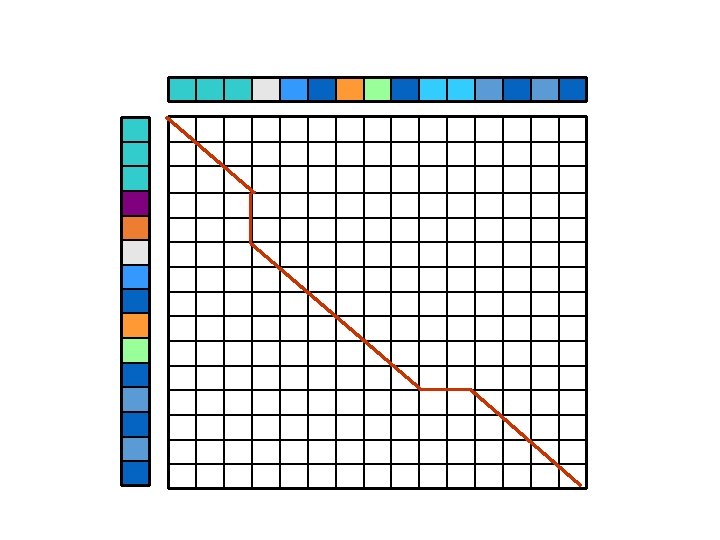
Stereo with dynamic programming • Shortest path in a grid • Diagonals: constant disparity • Moving along the diagonal – pay unary cost (cost of pixel match) • Move sideways – pay binary cost, i. e. disparity change (occlusion, right or left) • Cost prefers fronto-parallel planes. Penalty is paid for tilted planes

Dynamic programming on a grid Start

Dynamic programming: pros and cons • Advantages: • Simple, efficient • Achieves global optimum • Generally works well

Dynamic programming: pros and cons • Advantages: • Simple, efficient • Achieves global optimum • Generally works well • Disadvantages: • Works separately on each epipolar line, does not enforce smoothness across epipolars • Prefers fronto-parallel planes • Too local? (considers only immediate neighbors)

Probability interpretation: the Viterbi algorithm •

Probability interpretation: the Viterbi algorithm •