EECS 252 Graduate Computer Architecture Lec 18 Storage

EECS 252 Graduate Computer Architecture Lec 18 – Storage David Patterson Electrical Engineering and Computer Sciences University of California, Berkeley http: //www. eecs. berkeley. edu/~pattrsn http: //vlsi. cs. berkeley. edu/cs 252 -s 06 CS 252 s 06 Storage

Review • Disks: Arial Density now 30%/yr vs. 100%/yr in 2000 s • TPC: price performance as normalizing configuration feature – Auditing to ensure no foul play – Throughput with restricted response time is normal measure • Fault Latent errors in system Failure in service • Components often fail slowly • Real systems: problems in maintenance, operation as well as hardware, software 9/25/2020 CS 252 s 06 Storage 2

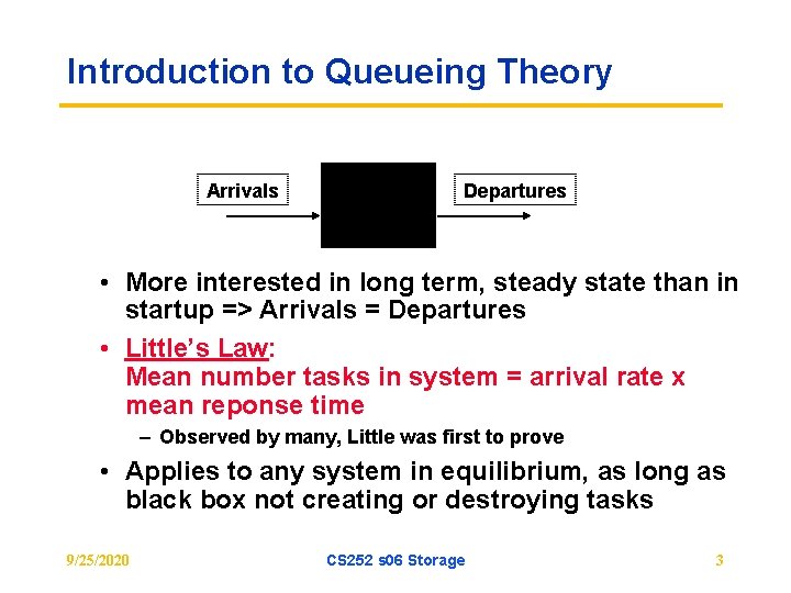
Introduction to Queueing Theory Arrivals Departures • More interested in long term, steady state than in startup => Arrivals = Departures • Little’s Law: Mean number tasks in system = arrival rate x mean reponse time – Observed by many, Little was first to prove • Applies to any system in equilibrium, as long as black box not creating or destroying tasks 9/25/2020 CS 252 s 06 Storage 3

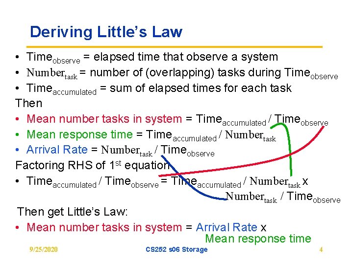
Deriving Little’s Law • Timeobserve = elapsed time that observe a system • Numbertask = number of (overlapping) tasks during Timeobserve • Timeaccumulated = sum of elapsed times for each task Then • Mean number tasks in system = Timeaccumulated / Timeobserve • Mean response time = Timeaccumulated / Numbertask • Arrival Rate = Numbertask / Timeobserve Factoring RHS of 1 st equation • Timeaccumulated / Timeobserve = Timeaccumulated / Numbertask x Numbertask / Timeobserve Then get Little’s Law: • Mean number tasks in system = Arrival Rate x Mean response time 9/25/2020 CS 252 s 06 Storage 4

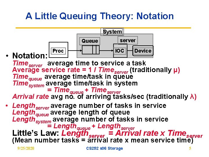
A Little Queuing Theory: Notation System Queue • Notation: Proc server IOC Device Timeserver average time to service a task Average service rate = 1 / Timeserver (traditionally µ) Timequeue average time/task in queue Timesystem average time/task in system = Timequeue + Timeserver Arrival rate avg no. of arriving tasks/sec (traditionally λ) • Lengthserver average number of tasks in service Lengthqueue average length of queue Lengthsystem average number of tasks in service = Lengthqueue + Lengthserver Little’s Law: Lengthserver = Arrival rate x Timeserver (Mean number tasks = arrival rate x mean service time) 9/25/2020 CS 252 s 06 Storage 5

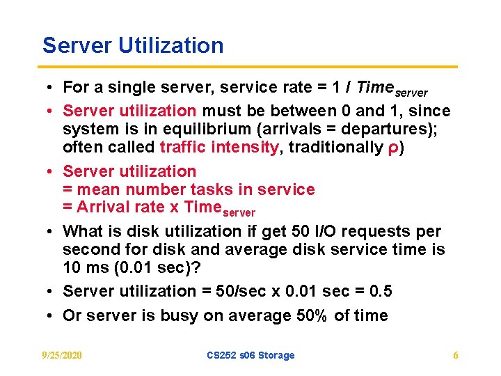
Server Utilization • For a single server, service rate = 1 / Timeserver • Server utilization must be between 0 and 1, since system is in equilibrium (arrivals = departures); often called traffic intensity, traditionally ρ) • Server utilization = mean number tasks in service = Arrival rate x Timeserver • What is disk utilization if get 50 I/O requests per second for disk and average disk service time is 10 ms (0. 01 sec)? • Server utilization = 50/sec x 0. 01 sec = 0. 5 • Or server is busy on average 50% of time 9/25/2020 CS 252 s 06 Storage 6

Time in Queue vs. Length of Queue • We assume First In First Out (FIFO) queue • Relationship of time in queue (Timequeue) to mean number of tasks in queue (Lengthqueue) ? • Timequeue = Lengthqueue x Timeserver + “Mean time to complete service of task when new task arrives if server is busy” • New task can arrive at any instant; how predict last part? • To predict performance, need to know sometime about distribution of events 9/25/2020 CS 252 s 06 Storage 7

Distribution of Random Variables • A variable is random if it takes one of a specified set of values with a specified probability – Cannot know exactly next value, but may know probability of all possible values • I/O Requests can be modeled by a random variable because OS normally switching between several processes generating independent I/O requests – Also given probabilistic nature of disks in seek and rotational delays • Can characterize distribution of values of a random variable with discrete values using a histogram – Divides range between the min & max values into buckets – Histograms then plot the number in each bucket as columns – Works for discrete values e. g. , number of I/O requests? • What about if not discrete? Very fine buckets 9/25/2020 CS 252 s 06 Storage 8

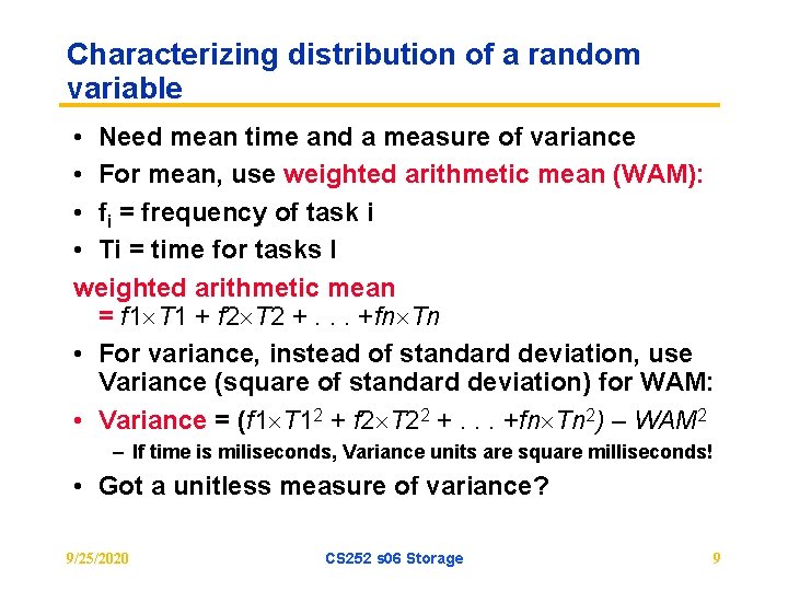
Characterizing distribution of a random variable • Need mean time and a measure of variance • For mean, use weighted arithmetic mean (WAM): • fi = frequency of task i • Ti = time for tasks I weighted arithmetic mean = f 1 T 1 + f 2 T 2 +. . . +fn Tn • For variance, instead of standard deviation, use Variance (square of standard deviation) for WAM: • Variance = (f 1 T 12 + f 2 T 22 +. . . +fn Tn 2) – WAM 2 – If time is miliseconds, Variance units are square milliseconds! • Got a unitless measure of variance? 9/25/2020 CS 252 s 06 Storage 9

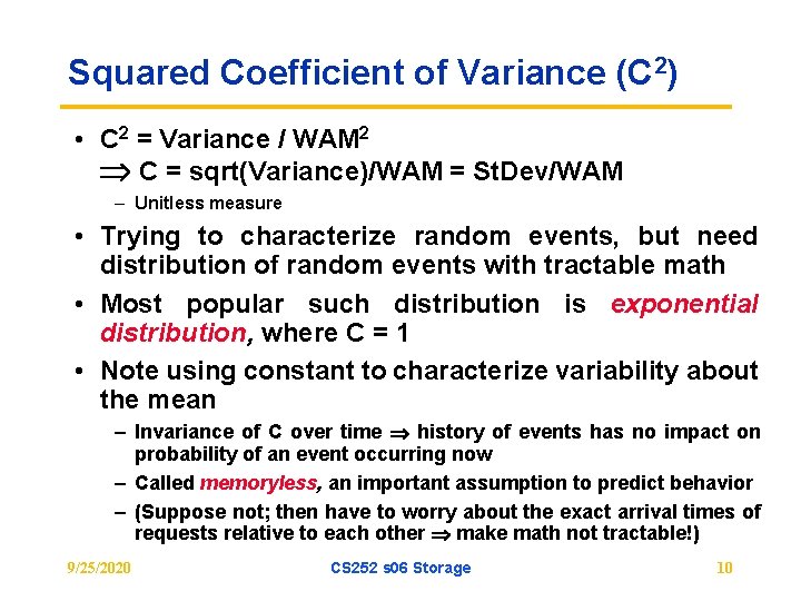
Squared Coefficient of Variance (C 2) • C 2 = Variance / WAM 2 C = sqrt(Variance)/WAM = St. Dev/WAM – Unitless measure • Trying to characterize random events, but need distribution of random events with tractable math • Most popular such distribution is exponential distribution, where C = 1 • Note using constant to characterize variability about the mean – Invariance of C over time history of events has no impact on probability of an event occurring now – Called memoryless, an important assumption to predict behavior – (Suppose not; then have to worry about the exact arrival times of requests relative to each other make math not tractable!) 9/25/2020 CS 252 s 06 Storage 10

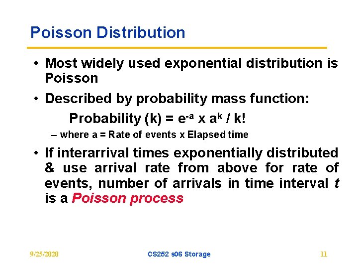
Poisson Distribution • Most widely used exponential distribution is Poisson • Described by probability mass function: Probability (k) = e-a x ak / k! – where a = Rate of events x Elapsed time • If interarrival times exponentially distributed & use arrival rate from above for rate of events, number of arrivals in time interval t is a Poisson process 9/25/2020 CS 252 s 06 Storage 11

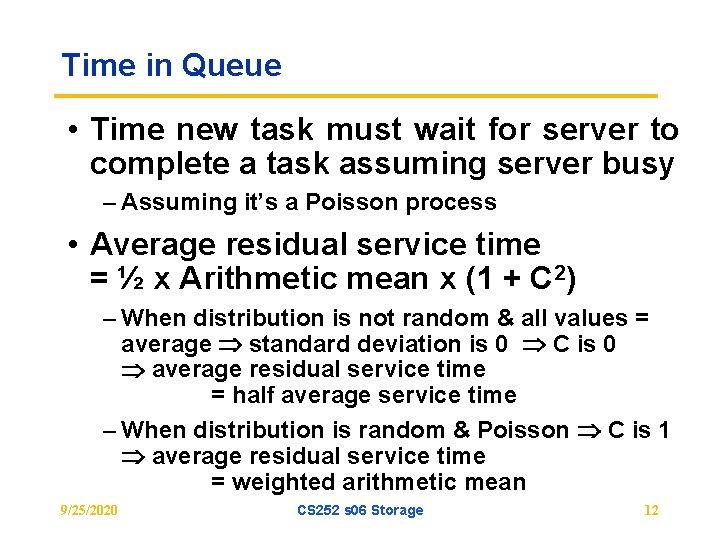
Time in Queue • Time new task must wait for server to complete a task assuming server busy – Assuming it’s a Poisson process • Average residual service time = ½ x Arithmetic mean x (1 + C 2) – When distribution is not random & all values = average standard deviation is 0 C is 0 average residual service time = half average service time – When distribution is random & Poisson C is 1 average residual service time = weighted arithmetic mean 9/25/2020 CS 252 s 06 Storage 12

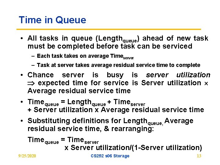
Time in Queue • All tasks in queue (Lengthqueue) ahead of new task must be completed before task can be serviced – Each task takes on average Timeserver – Task at server takes average residual service time to complete • Chance server is busy is server utilization expected time for service is Server utilization Average residual service time • Timequeue = Lengthqueue + Timeserver + Server utilization x Average residual service time • Substituting definitions for Lengthqueue, Average residual service time, & rearranging: Timequeue = Timeserver x Server utilization/(1 -Server utilization) 9/25/2020 CS 252 s 06 Storage 13

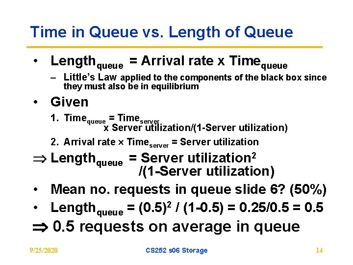
Time in Queue vs. Length of Queue • Lengthqueue = Arrival rate x Timequeue – Little’s Law applied to the components of the black box since they must also be in equilibrium • Given 1. Timequeue = Timeserver x Server utilization/(1 -Server utilization) 2. Arrival rate Timeserver = Server utilization Lengthqueue = Server utilization 2 /(1 -Server utilization) • Mean no. requests in queue slide 6? (50%) • Lengthqueue = (0. 5)2 / (1 -0. 5) = 0. 25/0. 5 = 0. 5 requests on average in queue 9/25/2020 CS 252 s 06 Storage 14

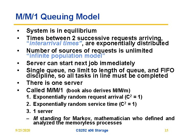
M/M/1 Queuing Model • • System is in equilibrium Times between 2 successive requests arriving, “interarrival times”, are exponentially distributed Number of sources of requests is unlimited “infinite population model” Server can start next job immediately Single queue, no limit to length of queue, and FIFO discipline, so all tasks in line must be completed There is one server Called M/M/1 (book also derives M/M/m) 1. 2. 3. – 9/25/2020 Exponentially random request arrival (C 2 = 1) Exponentially random service time (C 2 = 1) 1 server M standing for Markov, mathematician who defined analyzed the memoryless processes CS 252 s 06 Storage 15

CS 252: Administrivia • • Fun talking during Pizza last Wednesday Project Update Meeting Wednesday 4/19, 10 to 12: 30 – 635 Soda. Meeting signup online? • Monday 4/24 Quiz 2 5 -8 PM in room ? – (Mainly Ch 4 to 6) • • Wed 4/26 Bad Career Advice / Bad Talk Advice ? / Goodbye to Computer Architecture / Your Cal Cultural History Project Presentations Monday 5/1 (all day) Project Posters 5/3 Wednesday (11 -1 in Soda) Final Papers due Friday 5/5 – Email Archana, who will post papers on class web site 9/25/2020 CS 252 s 06 Storage 16

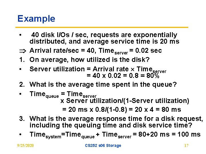
Example • 1. • 2. • 3. • 40 disk I/Os / sec, requests are exponentially distributed, and average service time is 20 ms Arrival rate/sec = 40, Timeserver = 0. 02 sec On average, how utilized is the disk? Server utilization = Arrival rate Timeserver = 40 x 0. 02 = 0. 8 = 80% What is the average time spent in the queue? Timequeue = Timeserver x Server utilization/(1 -Server utilization) = 20 ms x 0. 8/(1 -0. 8) = 20 x 4 = 80 ms What is the average response time for a disk request, including the queuing time and disk service time? Timesystem=Timequeue + Timeserver = 80+20 ms = 100 ms 9/25/2020 CS 252 s 06 Storage 17

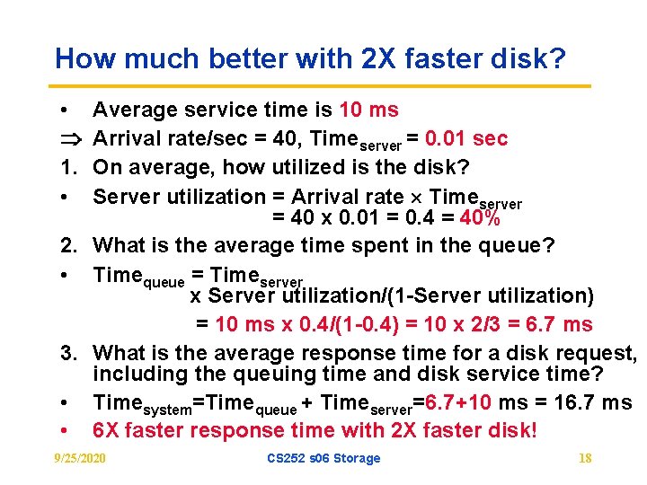
How much better with 2 X faster disk? • 1. • Average service time is 10 ms Arrival rate/sec = 40, Timeserver = 0. 01 sec On average, how utilized is the disk? Server utilization = Arrival rate Timeserver = 40 x 0. 01 = 0. 4 = 40% 2. What is the average time spent in the queue? • Timequeue = Timeserver x Server utilization/(1 -Server utilization) = 10 ms x 0. 4/(1 -0. 4) = 10 x 2/3 = 6. 7 ms 3. What is the average response time for a disk request, including the queuing time and disk service time? • Timesystem=Timequeue + Timeserver=6. 7+10 ms = 16. 7 ms • 6 X faster response time with 2 X faster disk! 9/25/2020 CS 252 s 06 Storage 18

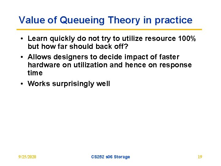
Value of Queueing Theory in practice • Learn quickly do not try to utilize resource 100% but how far should back off? • Allows designers to decide impact of faster hardware on utilization and hence on response time • Works surprisingly well 9/25/2020 CS 252 s 06 Storage 19

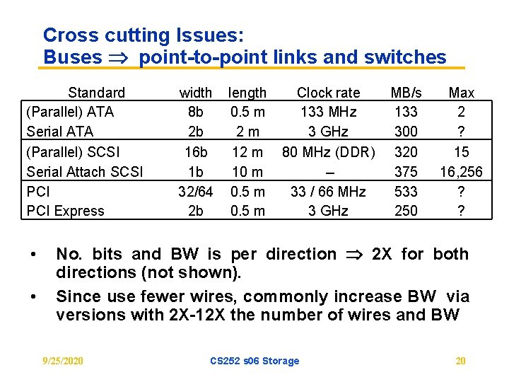
Cross cutting Issues: Buses point-to-point links and switches Standard (Parallel) ATA Serial ATA (Parallel) SCSI Serial Attach SCSI PCI Express • • width 8 b 2 b 16 b 1 b 32/64 2 b length 0. 5 m 2 m 12 m 10 m 0. 5 m Clock rate 133 MHz 3 GHz 80 MHz (DDR) -33 / 66 MHz 3 GHz MB/s 133 300 320 375 533 250 Max 2 ? 15 16, 256 ? ? No. bits and BW is per direction 2 X for both directions (not shown). Since use fewer wires, commonly increase BW via versions with 2 X-12 X the number of wires and BW 9/25/2020 CS 252 s 06 Storage 20

Storage Example: Internet Archive • Goal of making a historical record of the Internet – Internet Archive began in 1996 – Wayback Machine interface perform time travel to see what the website at a URL looked like in the past • It contains over a petabyte (1015 bytes), and is growing by 20 terabytes (1012 bytes) of new data per month • In addition to storing the historical record, the same hardware is used to crawl the Web every few months to get snapshots of the Interne. 9/25/2020 CS 252 s 06 Storage 21

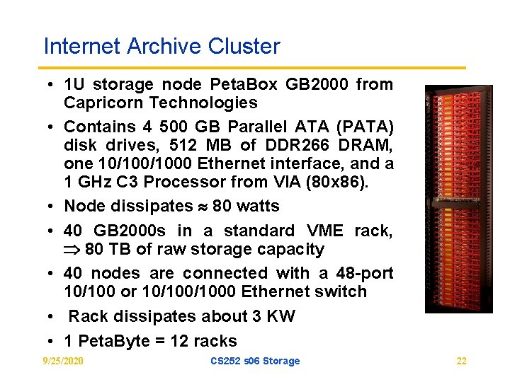
Internet Archive Cluster • 1 U storage node Peta. Box GB 2000 from Capricorn Technologies • Contains 4 500 GB Parallel ATA (PATA) disk drives, 512 MB of DDR 266 DRAM, one 10/1000 Ethernet interface, and a 1 GHz C 3 Processor from VIA (80 x 86). • Node dissipates 80 watts • 40 GB 2000 s in a standard VME rack, 80 TB of raw storage capacity • 40 nodes are connected with a 48 -port 10/100 or 10/1000 Ethernet switch • Rack dissipates about 3 KW • 1 Peta. Byte = 12 racks 9/25/2020 CS 252 s 06 Storage 22

Estimated Cost • Via processor, 512 MB of DDR 266 DRAM, ATA disk controller, power supply, fans, and enclosure = $500 • 7200 RPM Parallel ATA drives holds 500 GB = $375. • 48 -port 10/1000 Ethernet switch and all cables for a rack = $3000. • Cost $84, 500 for a 80 -TB rack. • 160 Disks are 60% of the cost 9/25/2020 CS 252 s 06 Storage 23

Estimated Performance • 7200 RPM Parallel ATA drives holds 500 GB, has an average time seek of 8. 5 ms, transfers at 50 MB/second from the disk. The PATA link speed is 133 MB/second. – performance of the VIA processor is 1000 MIPS. – operating system uses 50, 000 CPU instructions for a disk I/O. – network protocol stacks uses 100, 000 CPU instructions to transmit a data block between the cluster and the external world • ATA controller overhead is 0. 1 ms to perform a disk I/O. • Average I/O size is 16 KB for accesses to the historical record via the Wayback interface, and 50 KB when collecting a new snapshot • Disks are limit: 75 I/Os/s per disk, 300/s per node, 12000/s per rack, or about 200 to 600 Mbytes / sec Bandwidth per rack • Switch needs to support 1. 6 to 3. 8 Gbits/second over 40 Gbit/sec links 9/25/2020 CS 252 s 06 Storage 24

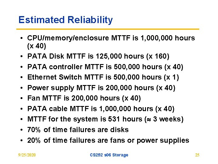
Estimated Reliability • CPU/memory/enclosure MTTF is 1, 000 hours (x 40) • PATA Disk MTTF is 125, 000 hours (x 160) • PATA controller MTTF is 500, 000 hours (x 40) • Ethernet Switch MTTF is 500, 000 hours (x 1) • Power supply MTTF is 200, 000 hours (x 40) • Fan MTTF is 200, 000 hours (x 40) • PATA cable MTTF is 1, 000 hours (x 40) • MTTF for the system is 531 hours ( 3 weeks) • 70% of time failures are disks • 20% of time failures are fans or power supplies 9/25/2020 CS 252 s 06 Storage 25

RAID Paper Discussion • • • What was main motivation for RAID in paper? Did prediction of processor performance and disk capacity hold? What were the performance figures of merit to compare RAID levels? What RAID groups sizes were in the paper? Are they realistic? Why would RAID 2 (ECC) have lower predicted MTTF than RAID 3 (Parity)? 9/25/2020 CS 252 s 06 Storage 26

RAID Paper Discussion • • • How propose balance performance and capacity of RAID 1 to RAID 5? What do you think of it? What were some of the open issues? Which were significant? In retrospect, what do you think were important contributions? What did the authors get wrong? In retrospect: – – – 9/25/2020 RAID in Hardware vs. RAID in Software Rated MTTF vs. in the field Synchronization of disks in an array EMC ($10 B sales in 2005) and RAID Who invented RAID? CS 252 s 06 Storage 27

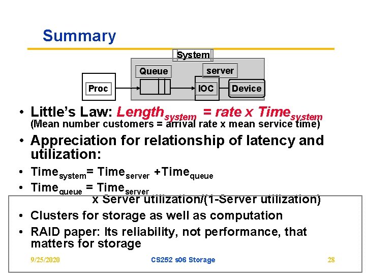
Summary System Queue Proc server IOC Device • Little’s Law: Lengthsystem = rate x Timesystem (Mean number customers = arrival rate x mean service time) • Appreciation for relationship of latency and utilization: • Timesystem= Timeserver +Timequeue • Timequeue = Timeserver x Server utilization/(1 -Server utilization) • Clusters for storage as well as computation • RAID paper: Its reliability, not performance, that matters for storage 9/25/2020 CS 252 s 06 Storage 28