EE 313 Linear Systems and Signals Fall 2018

EE 313 Linear Systems and Signals Fall 2018 Sampling and Aliasing Prof. Brian L. Evans Dept. of Electrical and Computer Engineering The University of Texas at Austin Textbook: Mc. Clellan, Schafer & Yoder, Signal Processing First, 2003 Lecture 5 http: //www. ece. utexas. edu/~bevans/courses/signals

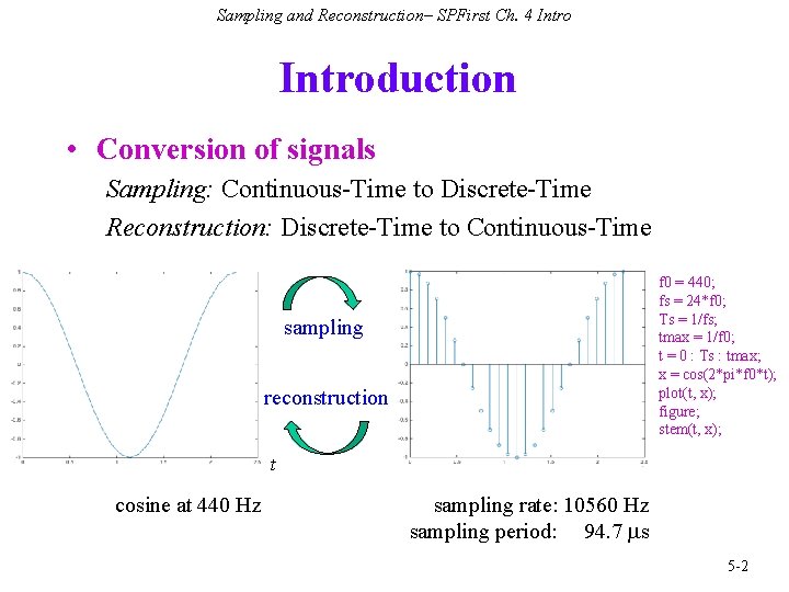
Sampling and Reconstruction– SPFirst Ch. 4 Introduction • Conversion of signals Sampling: Continuous-Time to Discrete-Time Reconstruction: Discrete-Time to Continuous-Time f 0 = 440; fs = 24*f 0; Ts = 1/fs; tmax = 1/f 0; t = 0 : Ts : tmax; x = cos(2*pi*f 0*t); plot(t, x); figure; stem(t, x); sampling reconstruction t cosine at 440 Hz sampling rate: 10560 Hz sampling period: 94. 7 ms 5 -2

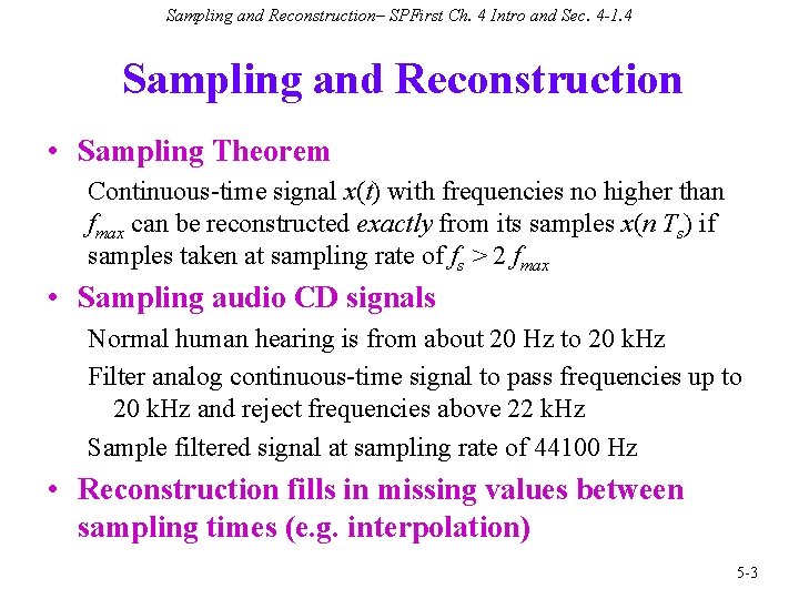
Sampling and Reconstruction– SPFirst Ch. 4 Intro and Sec. 4 -1. 4 Sampling and Reconstruction • Sampling Theorem Continuous-time signal x(t) with frequencies no higher than fmax can be reconstructed exactly from its samples x(n Ts) if samples taken at sampling rate of fs > 2 fmax • Sampling audio CD signals Normal human hearing is from about 20 Hz to 20 k. Hz Filter analog continuous-time signal to pass frequencies up to 20 k. Hz and reject frequencies above 22 k. Hz Sample filtered signal at sampling rate of 44100 Hz • Reconstruction fills in missing values between sampling times (e. g. interpolation) 5 -3

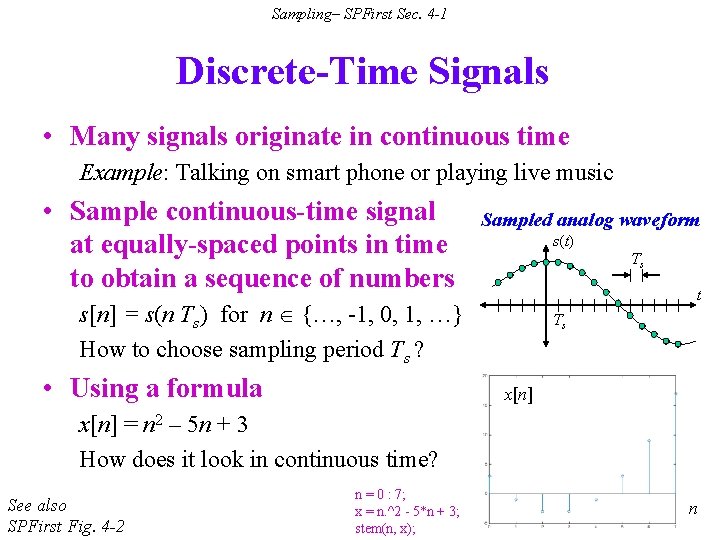
Sampling– SPFirst Sec. 4 -1 Discrete-Time Signals • Many signals originate in continuous time Example: Talking on smart phone or playing live music • Sample continuous-time signal at equally-spaced points in time to obtain a sequence of numbers Sampled analog waveform s(t) Ts t s[n] = s(n Ts) for n {…, -1, 0, 1, …} How to choose sampling period Ts ? • Using a formula Ts x[n] = n 2 – 5 n + 3 How does it look in continuous time? See also SPFirst Fig. 4 -2 n = 0 : 7; x = n. ^2 - 5*n + 3; stem(n, x); 5 -4 n

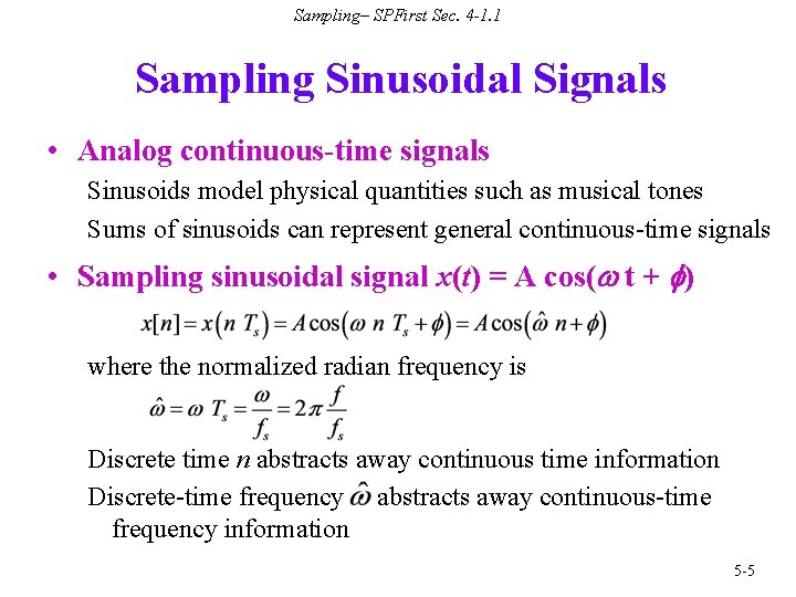
Sampling– SPFirst Sec. 4 -1. 1 Sampling Sinusoidal Signals • Analog continuous-time signals Sinusoids model physical quantities such as musical tones Sums of sinusoids can represent general continuous-time signals • Sampling sinusoidal signal x(t) = A cos(w t + f) where the normalized radian frequency is Discrete time n abstracts away continuous time information Discrete-time frequency abstracts away continuous-time frequency information 5 -5

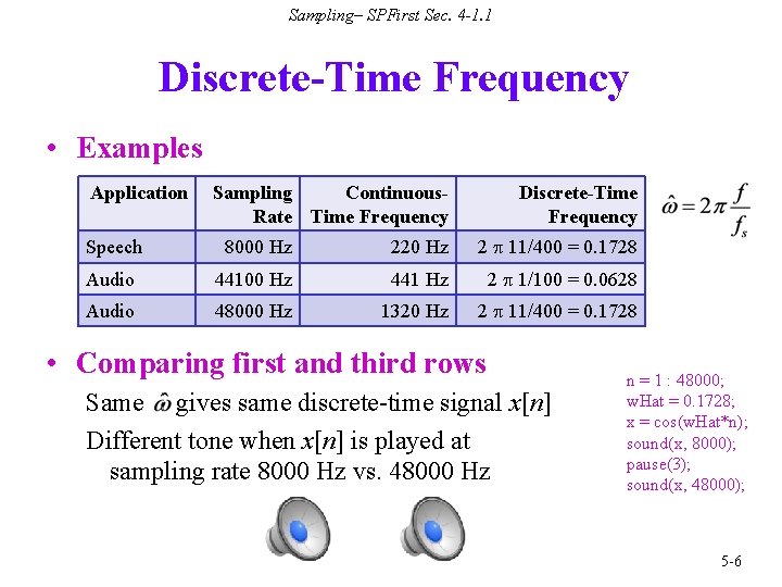
Sampling– SPFirst Sec. 4 -1. 1 Discrete-Time Frequency • Examples Application Sampling Continuous. Rate Time Frequency Discrete-Time Frequency Speech 8000 Hz 220 Hz 2 p 11/400 = 0. 1728 Audio 44100 Hz 441 Hz 2 p 1/100 = 0. 0628 Audio 48000 Hz 1320 Hz 2 p 11/400 = 0. 1728 • Comparing first and third rows Same gives same discrete-time signal x[n] Different tone when x[n] is played at sampling rate 8000 Hz vs. 48000 Hz n = 1 : 48000; w. Hat = 0. 1728; x = cos(w. Hat*n); sound(x, 8000); pause(3); sound(x, 48000); 5 -6

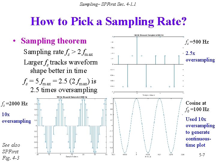
Sampling– SPFirst Sec. 4 -1. 1 How to Pick a Sampling Rate? • Sampling theorem Sampling rate fs > 2 fmax Larger fs tracks waveform shape better in time fs = 5 fmax = 2. 5 (2 fmax) is 2. 5 times oversampling fs =2000 Hz 10 x oversampling See also SPFirst Fig. 4 -3 fs =500 Hz 2. 5 x oversampling Cosine at f 0 =100 Hz Used 10 x oversampling to generate continuoustime plot 5 -7

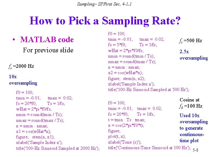
Sampling– SPFirst Sec. 4 -1. 1 How to Pick a Sampling Rate? • MATLAB code For previous slide fs =2000 Hz 10 x oversampling f 0 = 100; tmin = -0. 01; tmax = 0. 02; fs = 20*f 0; Ts = 1/fs; w. Hat = 2*pi*f 0/fs; nmin = round(tmin / Ts); nmax = round(tmax / Ts); n = nmin : nmax; x 1 = cos(w. Hat*n); figure; stem(n, x 1); xlabel('Sample Index n'); title('100 -Hz Sinusoid Sampled at 2000 Hz'); f 0 = 100; tmin = -0. 01; tmax = 0. 02; fs =500 Hz fs = 5*f 0; Ts = 1/fs; w. Hat = 2*pi*f 0/fs; 2. 5 x nmin = round(tmin / Ts); oversampling nmax = round(tmax / Ts); n = nmin : nmax; x 2 = cos(w. Hat*n); figure; stem(n, x 2); xlabel('Sample Index n'); title('100 -Hz Sinusoid Sampled at 500 Hz'); Cosine at f 0 = 100; f 0 =100 Hz tmin = -0. 01; tmax = 0. 02; fs = 20*f 0; Ts = 1/fs; Used 10 x t = tmin : Ts : tmax; oversampling x = cos(2*pi*f 0*t); to generate figure; continuousplot(t, x); time plot xlabel('Time (s)'); title('Continuous-Time Sinusoid at 100 Hz'); 5 -8

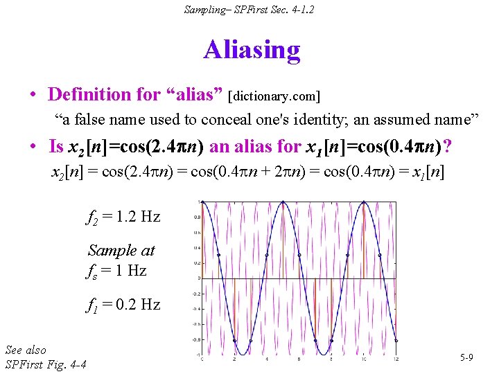
Sampling– SPFirst Sec. 4 -1. 2 Aliasing • Definition for “alias” [dictionary. com] “a false name used to conceal one's identity; an assumed name” • Is x 2[n]=cos(2. 4 pn) an alias for x 1[n]=cos(0. 4 pn)? x 2[n] = cos(2. 4 pn) = cos(0. 4 pn + 2 pn) = cos(0. 4 pn) = x 1[n] f 2 = 1. 2 Hz Sample at fs = 1 Hz f 1 = 0. 2 Hz See also SPFirst Fig. 4 -4 5 -9

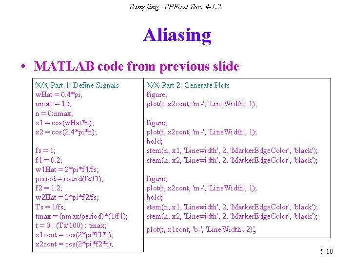
Sampling– SPFirst Sec. 4 -1. 2 Aliasing • MATLAB code from previous slide %% Part 1: Define Signals w. Hat = 0. 4*pi; nmax = 12; n = 0: nmax; x 1 = cos(w. Hat*n); x 2 = cos(2. 4*pi*n); fs = 1; f 1 = 0. 2; w 1 Hat = 2*pi*f 1/fs; period = round(fs/f 1); f 2 = 1. 2; w 2 Hat = 2*pi*f 2/fs; Ts = 1/fs; tmax = (nmax/period)*(1/f 1); t = 0 : (Ts/100) : tmax; x 1 cont = cos(2*pi*f 1*t); x 2 cont = cos(2*pi*f 2*t); %% Part 2: Generate Plots figure; plot(t, x 2 cont, 'm-', 'Line. Width', 1); hold; stem(n, x 1, 'Linewidth', 2, 'Marker. Edge. Color', 'black'); stem(n, x 2, 'Linewidth', 2, 'Marker. Edge. Color', 'black'); plot(t, x 1 cont, 'b-', 'Line. Width', 2); 5 -10

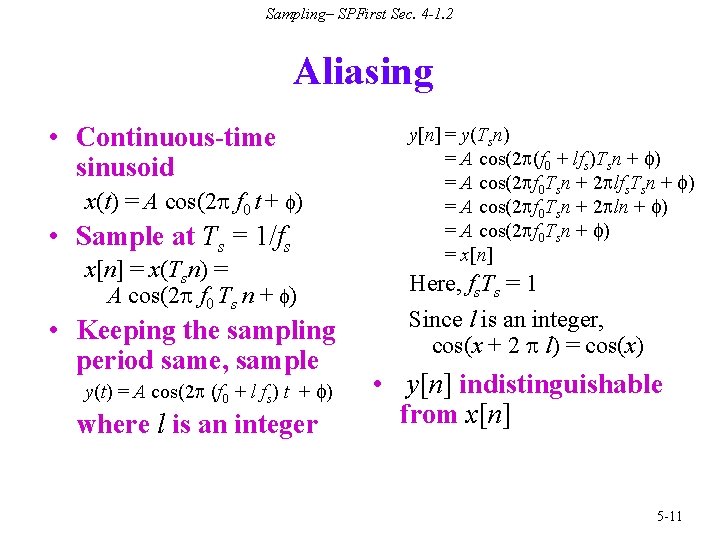
Sampling– SPFirst Sec. 4 -1. 2 Aliasing • Continuous-time sinusoid x(t) = A cos(2 p f 0 t + f) • Sample at Ts = 1/fs x[n] = x(Tsn) = A cos(2 p f 0 Ts n + f) • Keeping the sampling period same, sample y(t) = A cos(2 p (f 0 + l fs) t + f) where l is an integer y[n] = y(Tsn) = A cos(2 p(f 0 + lfs)Tsn + f) = A cos(2 pf 0 Tsn + 2 plfs. Tsn + f) = A cos(2 pf 0 Tsn + 2 pln + f) = A cos(2 pf 0 Tsn + f) = x[n] Here, fs. Ts = 1 Since l is an integer, cos(x + 2 p l) = cos(x) • y[n] indistinguishable from x[n] 5 -11

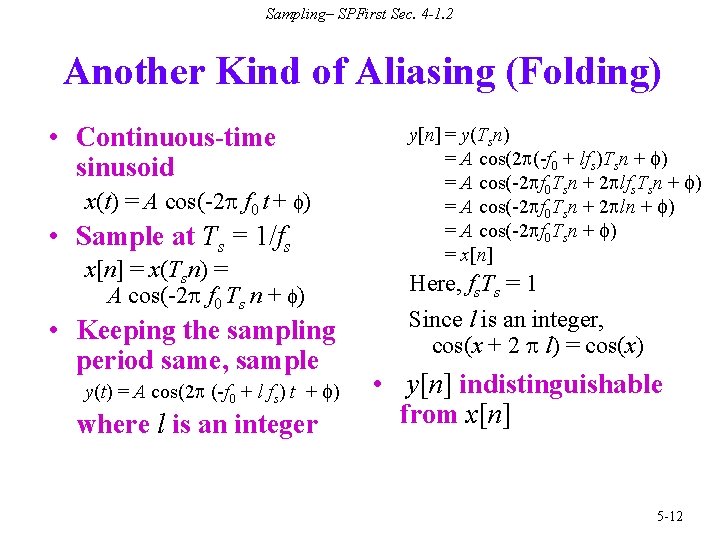
Sampling– SPFirst Sec. 4 -1. 2 Another Kind of Aliasing (Folding) • Continuous-time sinusoid x(t) = A cos(-2 p f 0 t + f) • Sample at Ts = 1/fs x[n] = x(Tsn) = A cos(-2 p f 0 Ts n + f) • Keeping the sampling period same, sample y(t) = A cos(2 p (-f 0 + l fs) t + f) where l is an integer y[n] = y(Tsn) = A cos(2 p(-f 0 + lfs)Tsn + f) = A cos(-2 pf 0 Tsn + 2 plfs. Tsn + f) = A cos(-2 pf 0 Tsn + 2 pln + f) = A cos(-2 pf 0 Tsn + f) = x[n] Here, fs. Ts = 1 Since l is an integer, cos(x + 2 p l) = cos(x) • y[n] indistinguishable from x[n] 5 -12

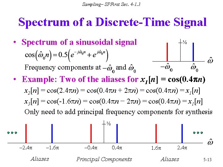
Sampling– SPFirst Sec. 4 -1. 3 Spectrum of a Discrete-Time Signal • Spectrum of a sinusoidal signal Frequency components at ½ and • Example: Two of the aliases for x 1[n] = cos(0. 4 pn) x 2[n] = cos(2. 4 pn) = cos(0. 4 pn + 2 pn) = cos(0. 4 pn) = x 1[n] x 3[n] = cos(-1. 6 pn) = cos(0. 4 pn − 2 pn) = cos(0. 4 pn) = x 1[n] Only need to add principal frequency components for synthesis ½ -2. 4 p -1. 6 p Aliases -0. 4 p Principal Components 1. 6 p 2. 4 p Aliases 5 -13

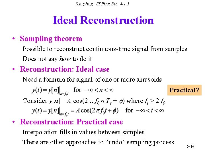
Sampling– SPFirst Sec. 4 -1. 5 Ideal Reconstruction • Sampling theorem Possible to reconstruct continuous-time signal from samples Does not say how to do it • Reconstruction: Ideal case Need a formula for signal of one or more sinusoids Practical? Consider y[n] = A cos(2 p f 0 n Ts + f) where fs > 2 f 0 • Reconstruction: Practical case Interpolation fills in values between samples There are other approaches to “undo” sampling process 5 -14

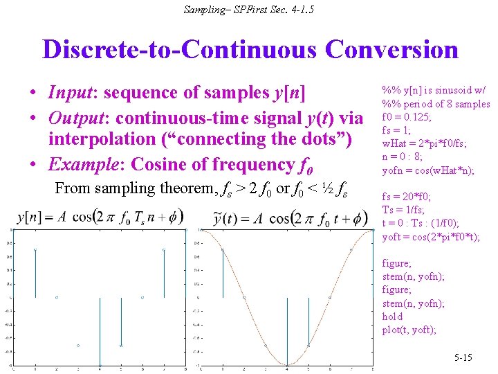
Sampling– SPFirst Sec. 4 -1. 5 Discrete-to-Continuous Conversion • Input: sequence of samples y[n] • Output: continuous-time signal y(t) via interpolation (“connecting the dots”) • Example: Cosine of frequency f 0 From sampling theorem, fs > 2 f 0 or f 0 < ½ fs %% y[n] is sinusoid w/ %% period of 8 samples f 0 = 0. 125; fs = 1; w. Hat = 2*pi*f 0/fs; n = 0 : 8; yofn = cos(w. Hat*n); fs = 20*f 0; Ts = 1/fs; t = 0 : Ts : (1/f 0); yoft = cos(2*pi*f 0*t); figure; stem(n, yofn); hold plot(t, yoft); 5 -15

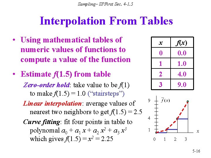
Sampling– SPFirst Sec. 4 -1. 5 Interpolation From Tables • Using mathematical tables of numeric values of functions to compute a value of the function • Estimate f(1. 5) from table Zero-order hold: take value to be f(1) to make f(1. 5) = 1. 0 (“stairsteps”) Linear interpolation: average values of nearest two neighbors to get f(1. 5) = 2. 5 Curve fitting: fit four points in table to polynomal a 0 + a 1 x + a 2 x 2 + a 3 x 3 which gives f(1. 5) = x 2 = 2. 25 x 0 1 2 f(x) 0. 0 1. 0 4. 0 3 9. 0 9 4 1 x 0 1 2 3 5 -16