ECECS 552 Pipelining to Superscalar Prof Mikko Lipasti

ECE/CS 552: Pipelining to Superscalar © Prof. Mikko Lipasti Lecture notes based in part on slides created by Mark Hill, David Wood, Guri Sohi, John Shen and Jim Smith

Pipelining to Superscalar • Forecast – Real pipelines – IBM RISC Experience – The case for superscalar – Instruction-level parallel machines – Superscalar pipeline organization – Superscalar pipeline design

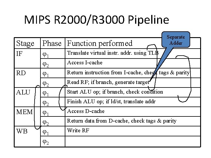
MIPS R 2000/R 3000 Pipeline Stage Phase Function performed IF RD ALU MEM WB φ1 φ2 φ1 φ2 Separate Adder Translate virtual instr. addr. using TLB Access I-cache Return instruction from I-cache, check tags & parity Read RF; if branch, generate target Start ALU op; if branch, check condition Finish ALU op; if ld/st, translate addr Access D-cache Return data from D-cache, check tags & parity Write RF

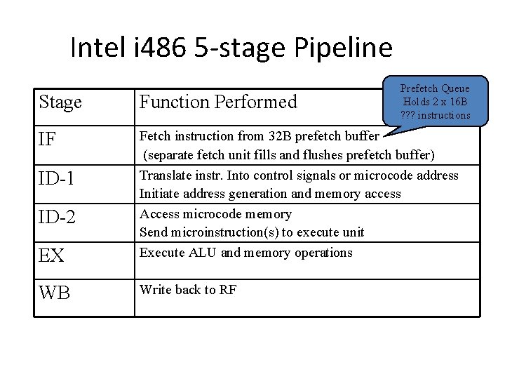
Intel i 486 5 -stage Pipeline Prefetch Queue Holds 2 x 16 B ? ? ? instructions Stage Function Performed IF EX Fetch instruction from 32 B prefetch buffer (separate fetch unit fills and flushes prefetch buffer) Translate instr. Into control signals or microcode address Initiate address generation and memory access Access microcode memory Send microinstruction(s) to execute unit Execute ALU and memory operations WB Write back to RF ID-1 ID-2

IBM RISC Experience [Agerwala and Cocke 1987] • Internal IBM study: Limits of a scalar pipeline? • Memory Bandwidth – Fetch 1 instr/cycle from I-cache – 40% of instructions are load/store (D-cache) • Code characteristics (dynamic) – – Loads – 25% Stores 15% ALU/RR – 40% Branches & jumps – 20% • 1/3 unconditional (always taken) • 1/3 conditional taken, 1/3 conditional not taken

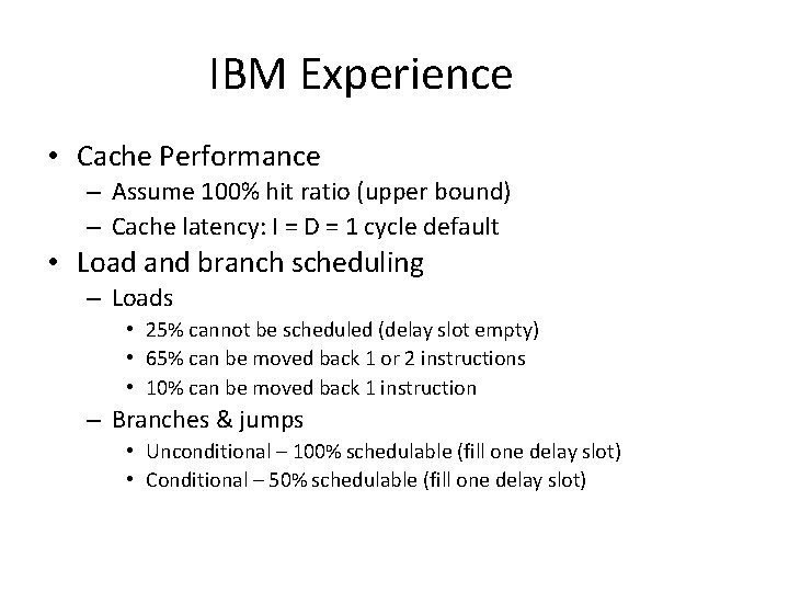
IBM Experience • Cache Performance – Assume 100% hit ratio (upper bound) – Cache latency: I = D = 1 cycle default • Load and branch scheduling – Loads • 25% cannot be scheduled (delay slot empty) • 65% can be moved back 1 or 2 instructions • 10% can be moved back 1 instruction – Branches & jumps • Unconditional – 100% schedulable (fill one delay slot) • Conditional – 50% schedulable (fill one delay slot)

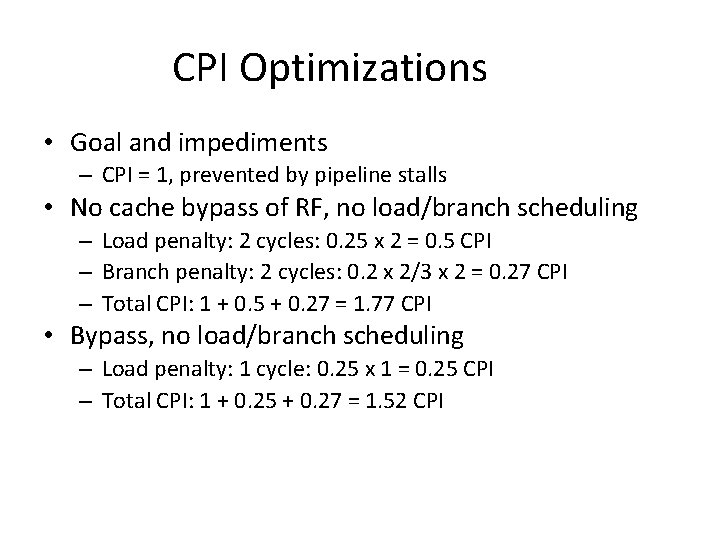
CPI Optimizations • Goal and impediments – CPI = 1, prevented by pipeline stalls • No cache bypass of RF, no load/branch scheduling – Load penalty: 2 cycles: 0. 25 x 2 = 0. 5 CPI – Branch penalty: 2 cycles: 0. 2 x 2/3 x 2 = 0. 27 CPI – Total CPI: 1 + 0. 5 + 0. 27 = 1. 77 CPI • Bypass, no load/branch scheduling – Load penalty: 1 cycle: 0. 25 x 1 = 0. 25 CPI – Total CPI: 1 + 0. 25 + 0. 27 = 1. 52 CPI

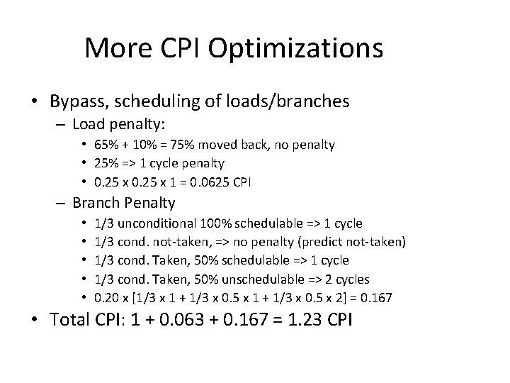
More CPI Optimizations • Bypass, scheduling of loads/branches – Load penalty: • 65% + 10% = 75% moved back, no penalty • 25% => 1 cycle penalty • 0. 25 x 1 = 0. 0625 CPI – Branch Penalty • • • 1/3 unconditional 100% schedulable => 1 cycle 1/3 cond. not-taken, => no penalty (predict not-taken) 1/3 cond. Taken, 50% schedulable => 1 cycle 1/3 cond. Taken, 50% unschedulable => 2 cycles 0. 20 x [1/3 x 1 + 1/3 x 0. 5 x 2] = 0. 167 • Total CPI: 1 + 0. 063 + 0. 167 = 1. 23 CPI

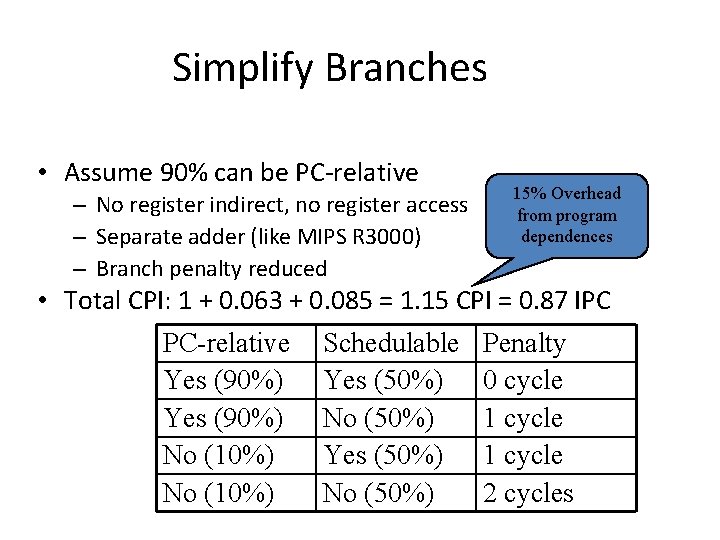
Simplify Branches • Assume 90% can be PC-relative – No register indirect, no register access – Separate adder (like MIPS R 3000) – Branch penalty reduced 15% Overhead from program dependences • Total CPI: 1 + 0. 063 + 0. 085 = 1. 15 CPI = 0. 87 IPC PC-relative Schedulable Penalty Yes (90%) Yes (50%) 0 cycle Yes (90%) No (50%) 1 cycle No (10%) Yes (50%) 1 cycle No (10%) No (50%) 2 cycles

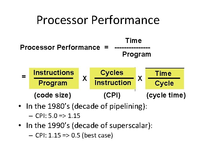
Processor Performance Time Processor Performance = -------Program = Instructions Program (code size) X Cycles X Instruction (CPI) Time Cycle (cycle time) • In the 1980’s (decade of pipelining): – CPI: 5. 0 => 1. 15 • In the 1990’s (decade of superscalar): – CPI: 1. 15 => 0. 5 (best case)

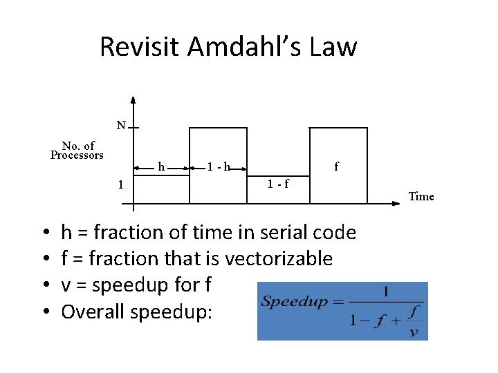
Revisit Amdahl’s Law N No. of Processors h 1 • • 1 -h f 1 -f h = fraction of time in serial code f = fraction that is vectorizable v = speedup for f Overall speedup: Time

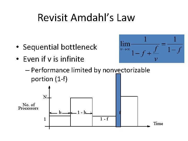
Revisit Amdahl’s Law • Sequential bottleneck • Even if v is infinite – Performance limited by nonvectorizable portion (1 -f) N No. of Processors h 1 1 -h f 1 -f Time

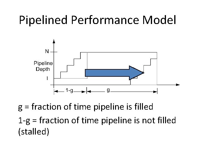
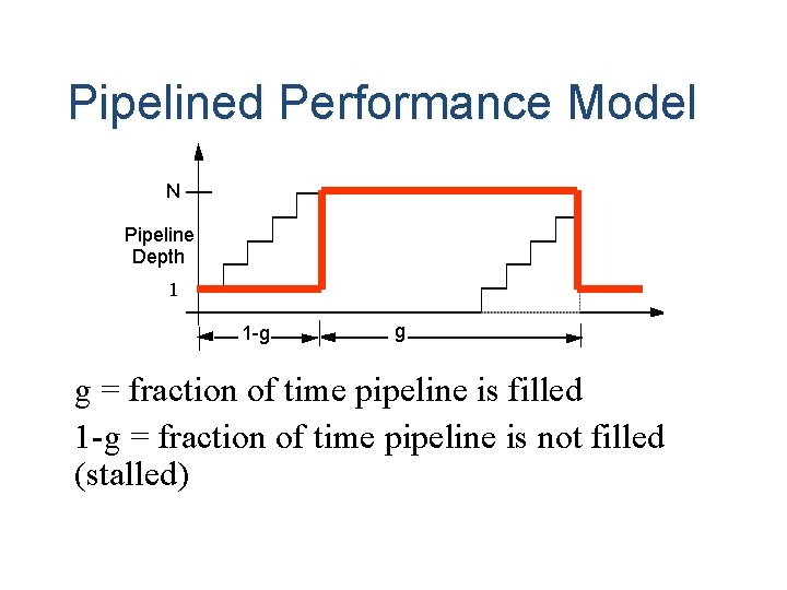
Pipelined Performance Model g = fraction of time pipeline is filled 1 -g = fraction of time pipeline is not filled (stalled)

Pipelined Performance Model N Pipeline Depth 1 1 -g g g = fraction of time pipeline is filled 1 -g = fraction of time pipeline is not filled (stalled)

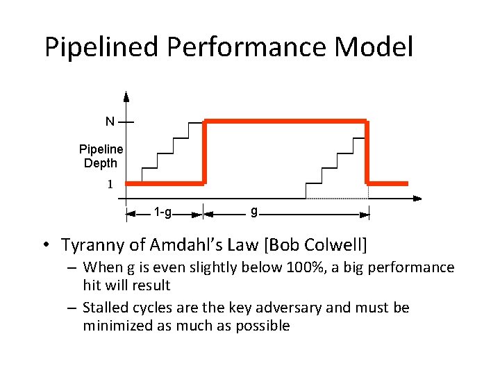
Pipelined Performance Model N Pipeline Depth 1 1 -g g • Tyranny of Amdahl’s Law [Bob Colwell] – When g is even slightly below 100%, a big performance hit will result – Stalled cycles are the key adversary and must be minimized as much as possible

Motivation for Superscalar [Agerwala and Cocke] Speedup jumps from 3 to 4. 3 for N=6, f=0. 8, but s =2 instead of s=1 (scalar) Typical Range

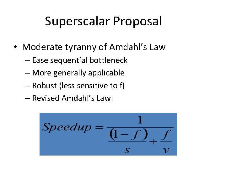
Superscalar Proposal • Moderate tyranny of Amdahl’s Law – Ease sequential bottleneck – More generally applicable – Robust (less sensitive to f) – Revised Amdahl’s Law:

Limits on Instruction Level Parallelism (ILP) Weiss and Smith [1984] 1. 58 Sohi and Vajapeyam [1987] 1. 81 Tjaden and Flynn [1970] 1. 86 (Flynn’s bottleneck) Tjaden and Flynn [1973] 1. 96 Uht [1986] 2. 00 Smith et al. [1989] 2. 00 Jouppi and Wall [1988] 2. 40 Johnson [1991] 2. 50 Acosta et al. [1986] 2. 79 Wedig [1982] 3. 00 Butler et al. [1991] 5. 8 Melvin and Patt [1991] 6 Wall [1991] 7 (Jouppi disagreed) Kuck et al. [1972] 8 Riseman and Foster [1972] 51 (no control dependences) Nicolau and Fisher [1984] 90 (Fisher’s optimism)

Superscalar Proposal • Go beyond single instruction pipeline, achieve IPC > 1 • Dispatch multiple instructions per cycle • Provide more generally applicable form of concurrency (not just vectors) • Geared for sequential code that is hard to parallelize otherwise • Exploit fine-grained or instruction-level parallelism (ILP)

Classifying ILP Machines [Jouppi, DECWRL 1991] • Baseline scalar RISC – Issue parallelism = IP = 1 – Operation latency = OP = 1 – Peak IPC = 1

Classifying ILP Machines [Jouppi, DECWRL 1991] • Superpipelined: cycle time = 1/m of baseline – Issue parallelism = IP = 1 inst / minor cycle – Operation latency = OP = m minor cycles – Peak IPC = m instr / major cycle (m x speedup? )

Classifying ILP Machines [Jouppi, DECWRL 1991] • Superscalar: – Issue parallelism = IP = n inst / cycle – Operation latency = OP = 1 cycle – Peak IPC = n instr / cycle (n x speedup? )

Classifying ILP Machines [Jouppi, DECWRL 1991] • VLIW: Very Long Instruction Word – Issue parallelism = IP = n inst / cycle – Operation latency = OP = 1 cycle – Peak IPC = n instr / cycle = 1 VLIW / cycle

Classifying ILP Machines [Jouppi, DECWRL 1991] • Superpipelined-Superscalar – Issue parallelism = IP = n inst / minor cycle – Operation latency = OP = m minor cycles – Peak IPC = n x m instr / major cycle

Superscalar vs. Superpipelined • Roughly equivalent performance – If n = m then both have about the same IPC – Parallelism exposed in space vs. time

Superscalar Challenges