ECE 465 Petricks Algorithm for 2 level Minimization

ECE 465 Petrick’s Algorithm for 2 -level Minimization Shantanu Dutt University of Illinois at Chicago Acknowledgement: Transcribed to Powerpoint by Huan Ren from Prof. Shantanu Dutt’s handwritten notes

Petrick’s Algorithm for Choosing Minimal Cost cover l The PIT portion of Q-M can get optimal in most cases and near-optimal cost coverings, but will not be optimal in all cases. l Can use an optimal algebraic method called Petrick’s algorithm.

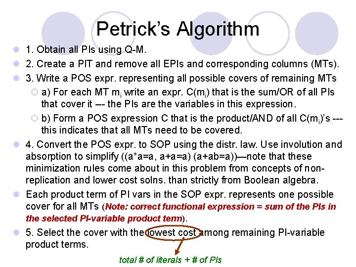
Petrick’s Algorithm l 1. Obtain all PIs using Q-M. l 2. Create a PIT and remove all EPIs and corresponding columns (MTs). l 3. Write a POS expr. representing all possible covers of remaining MTs ¡ a) For each MT mi write an expr. C(mi) that is the sum/OR of all PIs that cover it --- the PIs are the variables in this expression. ¡ b) Form a POS expression C that is the product/AND of all C(mi)’s --this indicates that all MTs need to be covered. l 4. Convert the POS expr. to SOP using the distr. law. Use involution and absorption to simplify ((a*a=a, a+a=a) (a+ab=a))—note that these minimization rules come about in this problem from concepts of nonreplication and lower cost solns. than strictly from Boolean algebra. l Each product term of PI vars in the SOP expr. represents one possible cover for all MTs (Note: correct functional expression = sum of the PIs in the selected PI-variable product term). l 5. Select the cover with the lowest cost among remaining PI-variable product terms. total # of literals + # of PIs

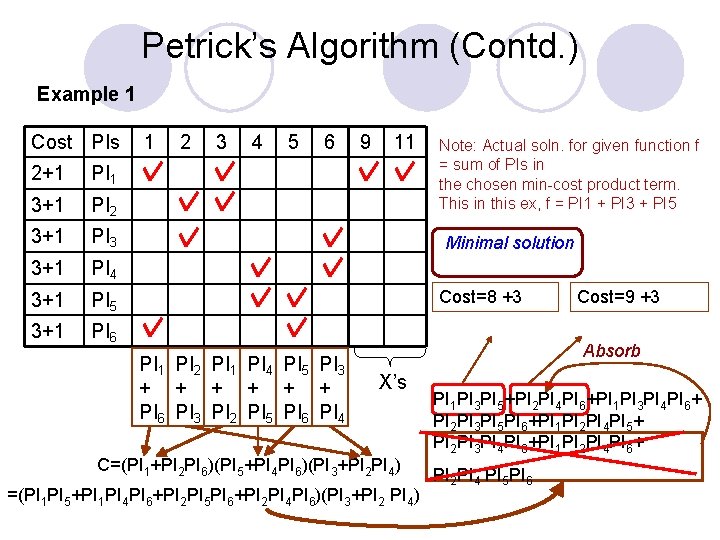
Petrick’s Algorithm (Contd. ) Example 1 Cost PIs 2+1 PI 1 3+1 PI 2 3+1 PI 3 3+1 PI 4 3+1 PI 5 3+1 PI 6 1 2 3 4 5 6 9 11 Note: Actual soln. for given function f = sum of PIs in the chosen min-cost product term. This in this ex, f = PI 1 + PI 3 + PI 5 Minimal solution Cost=8 +3 PI 1 PI 2 PI 1 PI 4 PI 5 PI 3 + + + PI 6 PI 3 PI 2 PI 5 PI 6 PI 4 Cost=9 +3 Absorb X’s C=(PI 1+PI 2 PI 6)(PI 5+PI 4 PI 6)(PI 3+PI 2 PI 4) =(PI 1 PI 5+PI 1 PI 4 PI 6+PI 2 PI 5 PI 6+PI 2 PI 4 PI 6)(PI 3+PI 2 PI 4) PI 1 PI 3 PI 5+PI 2 PI 4 PI 6+PI 1 PI 3 PI 4 PI 6+ PI 2 PI 3 PI 5 PI 6+PI 1 PI 2 PI 4 PI 5+ PI 2 PI 3 PI 4 PI 6+PI 1 PI 2 PI 4 PI 6+ PI 2 PI 4 PI 5 PI 6

Petrick’s Algorithm (Contd. ) l Exercise: Use this algorithm to obtain the least cover for the cyclic PIT problems in which we used the max. MT covering heuristic (Rule 3) to break the cycle.

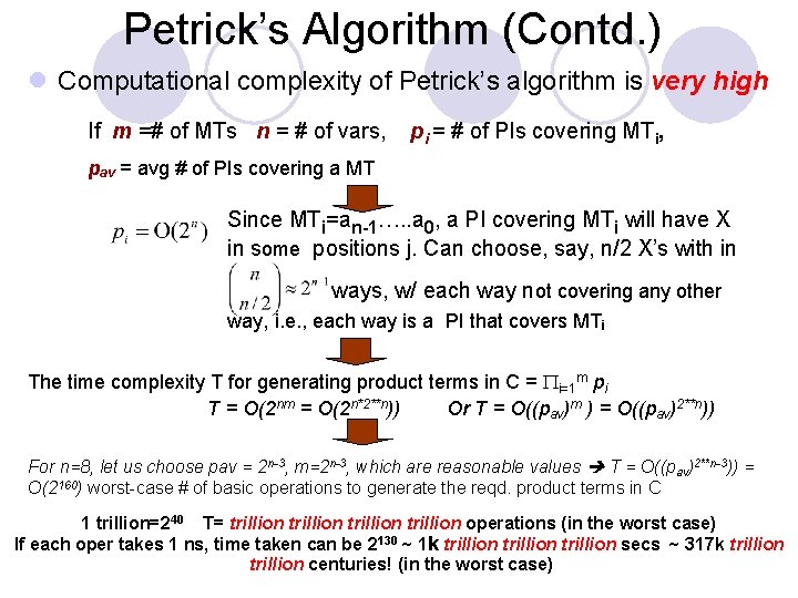
Petrick’s Algorithm (Contd. ) l Computational complexity of Petrick’s algorithm is very high If m =# of MTs n = # of vars, pi = # of PIs covering MTi, pav = avg # of PIs covering a MT Since MTi=an-1…. . a 0, a PI covering MTi will have X in some positions j. Can choose, say, n/2 X’s with in ways, w/ each way not covering any other way, i. e. , each way is a PI that covers MTi The time complexity T for generating product terms in C = Pi=1 m pi T = O(2 nm = O(2 n*2**n)) Or T = O((pav)m ) = O((pav)2**n)) For n=8, let us choose pav = 2 n-3, m=2 n-3, which are reasonable values T = O((pav)2**n-3)) = O(2160) worst-case # of basic operations to generate the reqd. product terms in C 1 trillion=240 T= trillion operations (in the worst case) If each oper takes 1 ns, time taken can be 2130 ~ 1 k trillion secs ~ 317 k trillion centuries! (in the worst case)

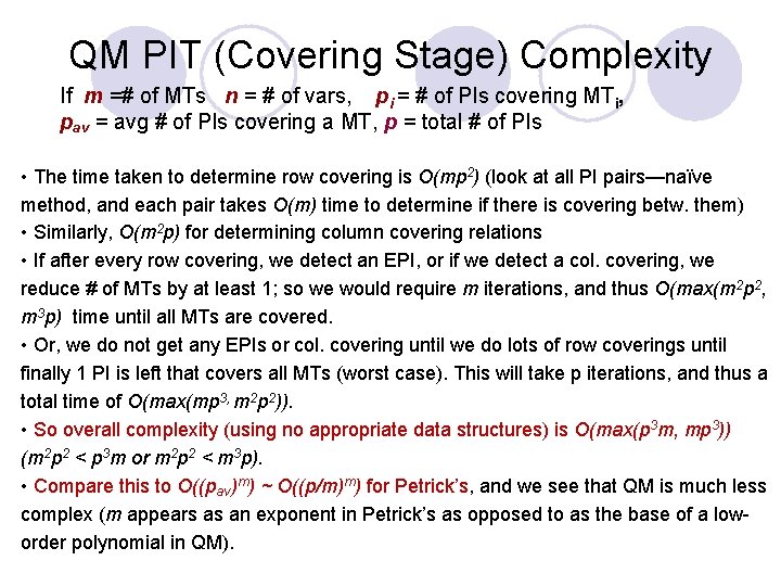
QM PIT (Covering Stage) Complexity If m =# of MTs n = # of vars, pi = # of PIs covering MTi, pav = avg # of PIs covering a MT, p = total # of PIs • The time taken to determine row covering is O(mp 2) (look at all PI pairs—naïve method, and each pair takes O(m) time to determine if there is covering betw. them) • Similarly, O(m 2 p) for determining column covering relations • If after every row covering, we detect an EPI, or if we detect a col. covering, we reduce # of MTs by at least 1; so we would require m iterations, and thus O(max(m 2 p 2, m 3 p) time until all MTs are covered. • Or, we do not get any EPIs or col. covering until we do lots of row coverings until finally 1 PI is left that covers all MTs (worst case). This will take p iterations, and thus a total time of O(max(mp 3, m 2 p 2)). • So overall complexity (using no appropriate data structures) is O(max(p 3 m, mp 3)) (m 2 p 2 < p 3 m or m 2 p 2 < m 3 p). • Compare this to O((pav)m) ~ O((p/m)m) for Petrick’s, and we see that QM is much less complex (m appears as an exponent in Petrick’s as opposed to as the base of a loworder polynomial in QM).

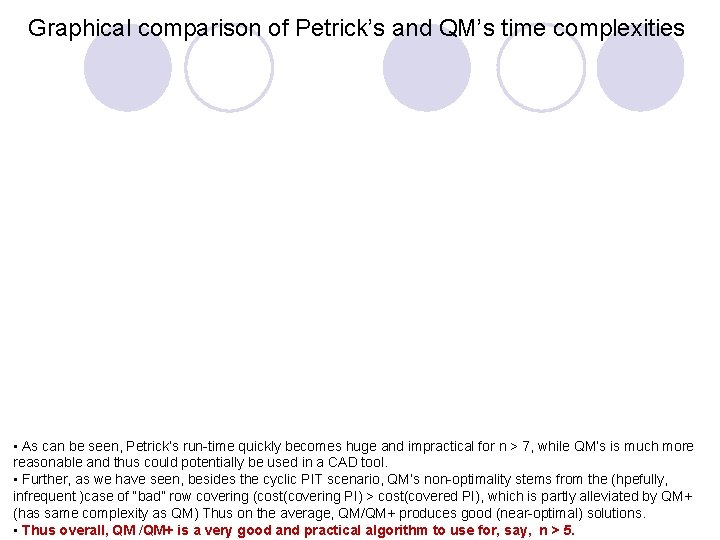
Graphical comparison of Petrick’s and QM’s time complexities • As can be seen, Petrick’s run-time quickly becomes huge and impractical for n > 7, while QM’s is much more reasonable and thus could potentially be used in a CAD tool. • Further, as we have seen, besides the cyclic PIT scenario, QM’s non-optimality stems from the (hpefully, infrequent )case of “bad” row covering (cost(covering PI) > cost(covered PI), which is partly alleviated by QM+ (has same complexity as QM) Thus on the average, QM/QM+ produces good (near-optimal) solutions. • Thus overall, QM /QM+ is a very good and practical algorithm to use for, say, n > 5.