Dynamic Programming 2004 Goodrich Tamassia Dynamic Programming 1

Dynamic Programming © 2004 Goodrich, Tamassia Dynamic Programming 1

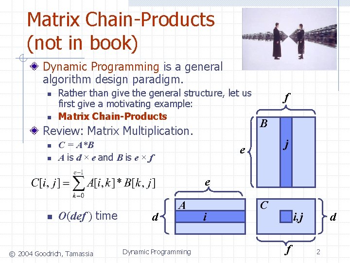
Matrix Chain-Products (not in book) Dynamic Programming is a general algorithm design paradigm. n n Rather than give the general structure, let us first give a motivating example: Matrix Chain-Products Review: Matrix Multiplication. n n C = A*B A is d × e and B is e × f f B j e e n O(def ) time © 2004 Goodrich, Tamassia d A Dynamic Programming i C i, j f d 2

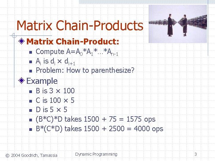
Matrix Chain-Products Matrix Chain-Product: n n n Compute A=A 0*A 1*…*An-1 Ai is di × di+1 Problem: How to parenthesize? Example n n n B is 3 × 100 C is 100 × 5 D is 5 × 5 (B*C)*D takes 1500 + 75 = 1575 ops B*(C*D) takes 1500 + 2500 = 4000 ops © 2004 Goodrich, Tamassia Dynamic Programming 3

An Enumeration Approach Matrix Chain-Product Alg. : n n n Try all possible ways to parenthesize A=A 0*A 1*…*An-1 Calculate number of ops for each one Pick the one that is best Running time: n n The number of paranethesizations is equal to the number of binary trees with n nodes This is exponential! It is called the Catalan number, and it is almost 4 n. This is a terrible algorithm! © 2004 Goodrich, Tamassia Dynamic Programming 4

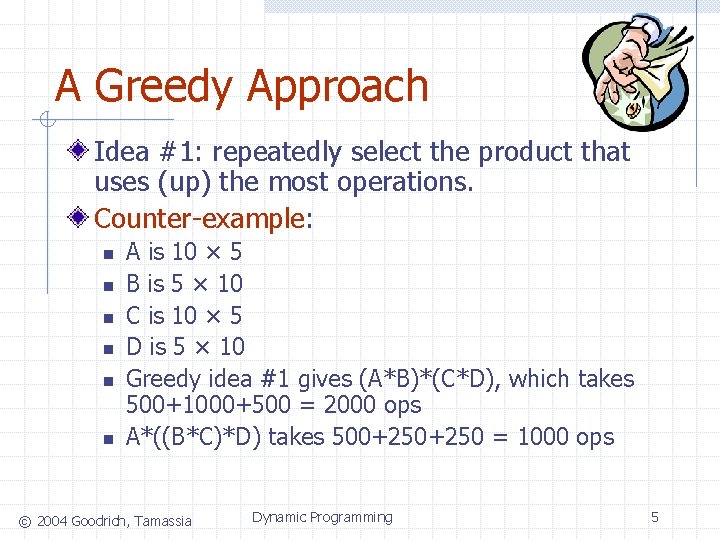
A Greedy Approach Idea #1: repeatedly select the product that uses (up) the most operations. Counter-example: n n n A is 10 × 5 B is 5 × 10 C is 10 × 5 D is 5 × 10 Greedy idea #1 gives (A*B)*(C*D), which takes 500+1000+500 = 2000 ops A*((B*C)*D) takes 500+250 = 1000 ops © 2004 Goodrich, Tamassia Dynamic Programming 5

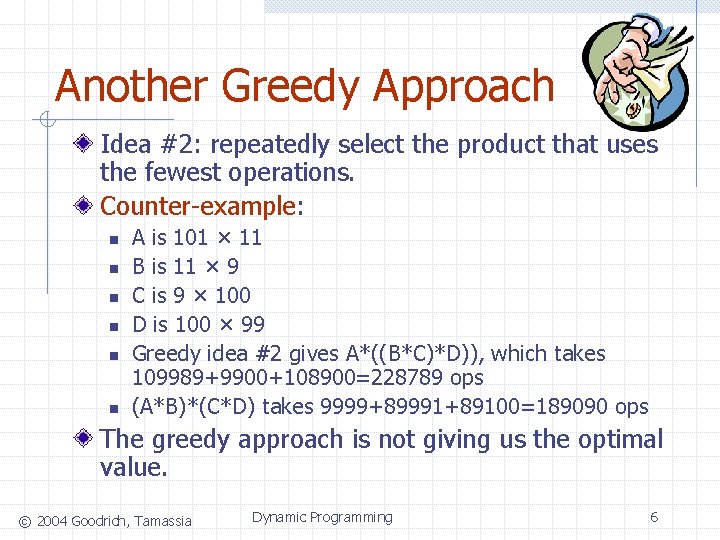
Another Greedy Approach Idea #2: repeatedly select the product that uses the fewest operations. Counter-example: n n n A is 101 × 11 B is 11 × 9 C is 9 × 100 D is 100 × 99 Greedy idea #2 gives A*((B*C)*D)), which takes 109989+9900+108900=228789 ops (A*B)*(C*D) takes 9999+89991+89100=189090 ops The greedy approach is not giving us the optimal value. © 2004 Goodrich, Tamassia Dynamic Programming 6

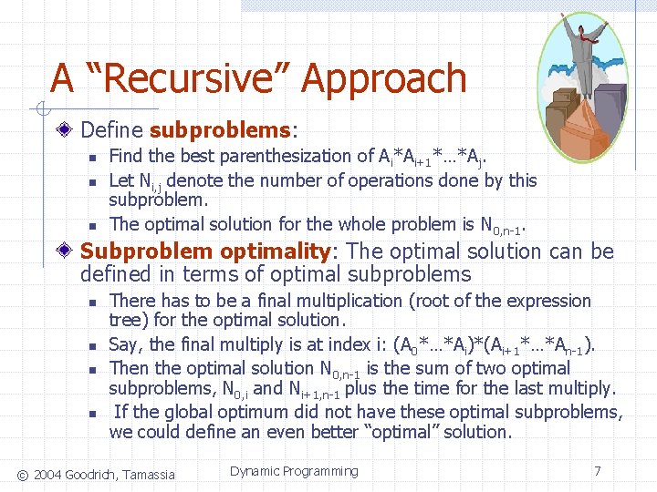
A “Recursive” Approach Define subproblems: n n n Find the best parenthesization of Ai*Ai+1*…*Aj. Let Ni, j denote the number of operations done by this subproblem. The optimal solution for the whole problem is N 0, n-1. Subproblem optimality: The optimal solution can be defined in terms of optimal subproblems n n There has to be a final multiplication (root of the expression tree) for the optimal solution. Say, the final multiply is at index i: (A 0*…*Ai)*(Ai+1*…*An-1). Then the optimal solution N 0, n-1 is the sum of two optimal subproblems, N 0, i and Ni+1, n-1 plus the time for the last multiply. If the global optimum did not have these optimal subproblems, we could define an even better “optimal” solution. © 2004 Goodrich, Tamassia Dynamic Programming 7

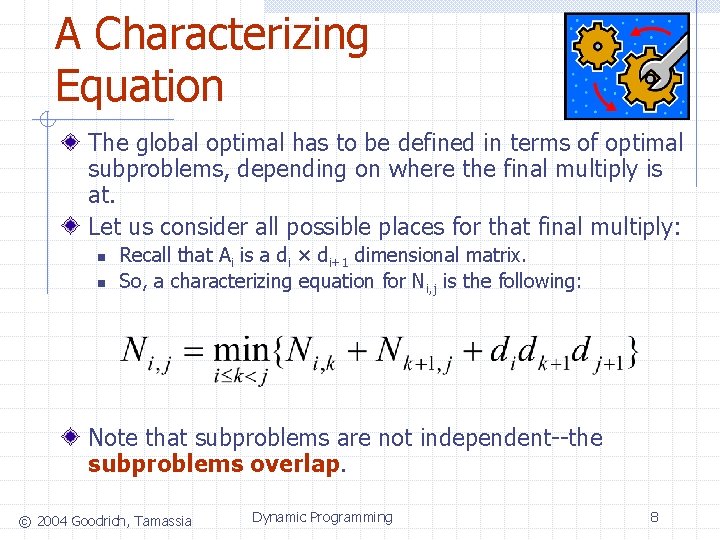
A Characterizing Equation The global optimal has to be defined in terms of optimal subproblems, depending on where the final multiply is at. Let us consider all possible places for that final multiply: n n Recall that Ai is a di × di+1 dimensional matrix. So, a characterizing equation for Ni, j is the following: Note that subproblems are not independent--the subproblems overlap. © 2004 Goodrich, Tamassia Dynamic Programming 8

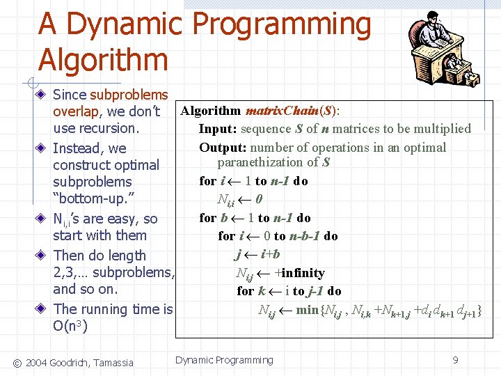
A Dynamic Programming Algorithm Since subproblems overlap, we don’t Algorithm matrix. Chain(S): Input: sequence S of n matrices to be multiplied use recursion. Output: number of operations in an optimal Instead, we paranethization of S construct optimal for i 1 to n-1 do subproblems Ni, i 0 “bottom-up. ” for b 1 to n-1 do Ni, i’s are easy, so for i 0 to n-b-1 do start with them j i+b Then do length Ni, j +infinity 2, 3, … subproblems, and so on. for k i to j-1 do Ni, j min{Ni, j , Ni, k +Nk+1, j +di dk+1 dj+1} The running time is O(n 3) © 2004 Goodrich, Tamassia Dynamic Programming 9

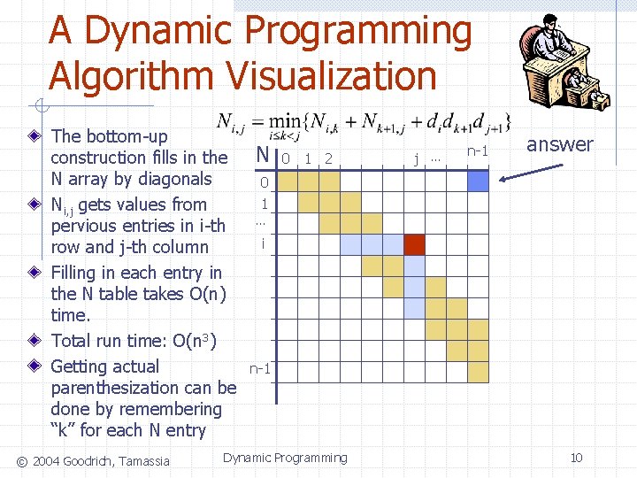
A Dynamic Programming Algorithm Visualization The bottom-up construction fills in the N array by diagonals Ni, j gets values from pervious entries in i-th row and j-th column Filling in each entry in the N table takes O(n) time. Total run time: O(n 3) Getting actual parenthesization can be done by remembering “k” for each N entry © 2004 Goodrich, Tamassia N 0 1 2 j … n-1 answer 0 1 … i n-1 Dynamic Programming 10

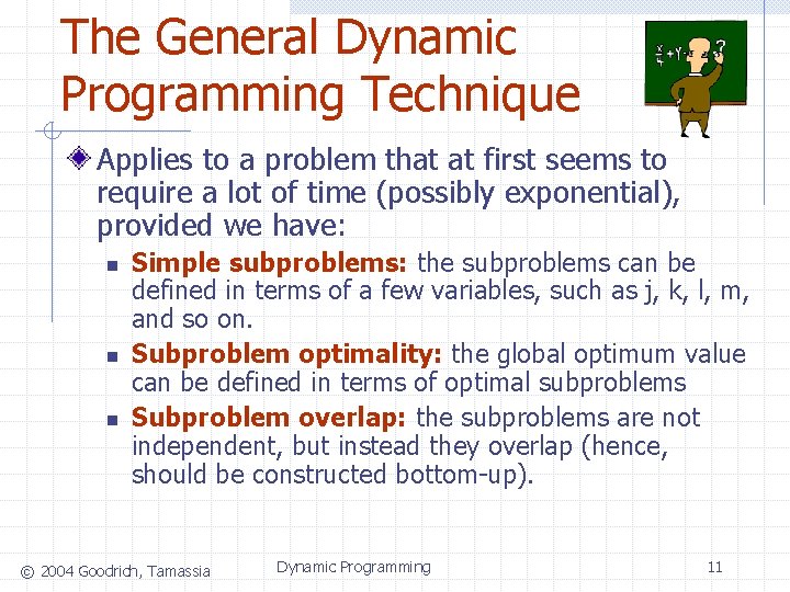
The General Dynamic Programming Technique Applies to a problem that at first seems to require a lot of time (possibly exponential), provided we have: n n n Simple subproblems: the subproblems can be defined in terms of a few variables, such as j, k, l, m, and so on. Subproblem optimality: the global optimum value can be defined in terms of optimal subproblems Subproblem overlap: the subproblems are not independent, but instead they overlap (hence, should be constructed bottom-up). © 2004 Goodrich, Tamassia Dynamic Programming 11

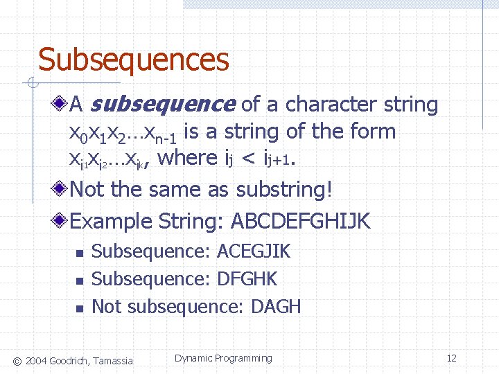
Subsequences A subsequence of a character string x 0 x 1 x 2…xn-1 is a string of the form xi xi …xi , where ij < ij+1. Not the same as substring! Example String: ABCDEFGHIJK 1 n n n 2 k Subsequence: ACEGJIK Subsequence: DFGHK Not subsequence: DAGH © 2004 Goodrich, Tamassia Dynamic Programming 12

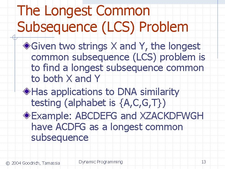
The Longest Common Subsequence (LCS) Problem Given two strings X and Y, the longest common subsequence (LCS) problem is to find a longest subsequence common to both X and Y Has applications to DNA similarity testing (alphabet is {A, C, G, T}) Example: ABCDEFG and XZACKDFWGH have ACDFG as a longest common subsequence © 2004 Goodrich, Tamassia Dynamic Programming 13

A Poor Approach to the LCS Problem A Brute-force solution: n n n Enumerate all subsequences of X Test which ones are also subsequences of Y Pick the longest one. Analysis: n n If X is of length n, then it has 2 n subsequences This is an exponential-time algorithm! © 2004 Goodrich, Tamassia Dynamic Programming 14

A Dynamic-Programming Approach to the LCS Problem Define L[i, j] to be the length of the longest common subsequence of X[0. . i] and Y[0. . j]. Allow for -1 as an index, so L[-1, k] = 0 and L[k, -1]=0, to indicate that the null part of X or Y has no match with the other. Then we can define L[i, j] in the general case as follows: 1. If xi=yj, then L[i, j] = L[i-1, j-1] + 1 (we can add this match) 2. If xi≠yj, then L[i, j] = max{L[i-1, j], L[i, j-1]} (we have no match here) Case 1: © 2004 Goodrich, Tamassia Dynamic Programming Case 2: 15

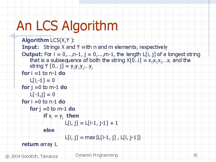
An LCS Algorithm LCS(X, Y ): Input: Strings X and Y with n and m elements, respectively Output: For i = 0, …, n-1, j = 0, . . . , m-1, the length L[i, j] of a longest string that is a subsequence of both the string X[0. . i] = x 0 x 1 x 2…xi and the string Y [0. . j] = y 0 y 1 y 2…yj for i =1 to n-1 do L[i, -1] = 0 for j =0 to m-1 do L[-1, j] = 0 for i =0 to n-1 do for j =0 to m-1 do if xi = yj then L[i, j] = L[i-1, j-1] + 1 else L[i, j] = max{L[i-1, j] , L[i, j-1]} return array L © 2004 Goodrich, Tamassia Dynamic Programming 16

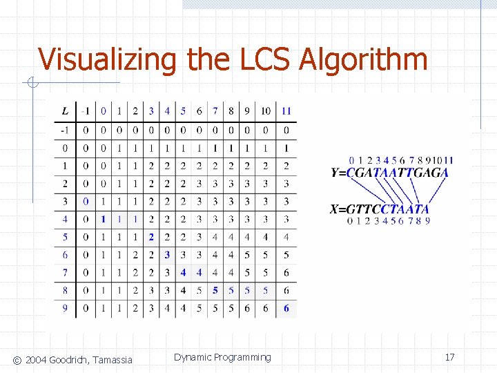
Visualizing the LCS Algorithm © 2004 Goodrich, Tamassia Dynamic Programming 17

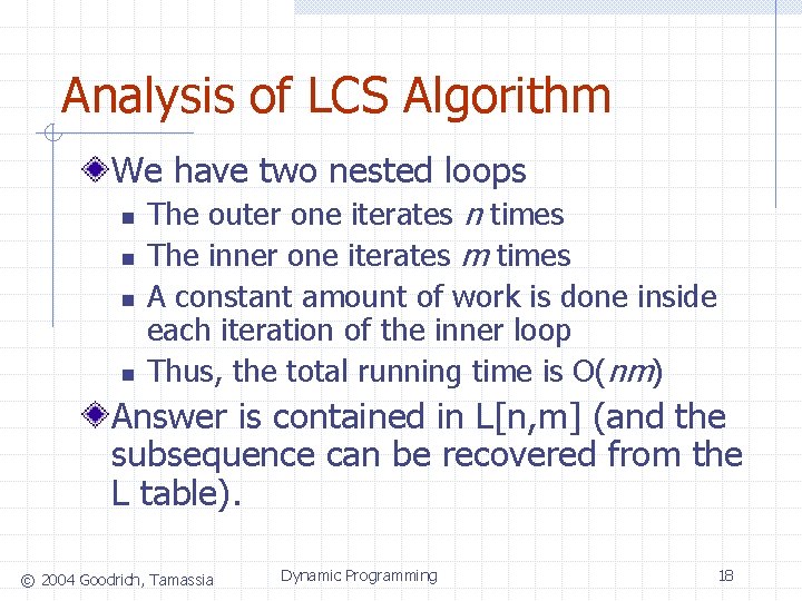
Analysis of LCS Algorithm We have two nested loops n n The outer one iterates n times The inner one iterates m times A constant amount of work is done inside each iteration of the inner loop Thus, the total running time is O(nm) Answer is contained in L[n, m] (and the subsequence can be recovered from the L table). © 2004 Goodrich, Tamassia Dynamic Programming 18