Data 100 Lecture 5 Data Cleaning Exploratory Data

Data 100 Lecture 5: Data Cleaning & Exploratory Data Analysis Slides by: Joseph E. Gonzalez, Deb Nolan, & Joe Hellerstein jegonzal@berkeley. edu deborah_nolan@berkeley. edu hellerstein@berkeley. edu ?

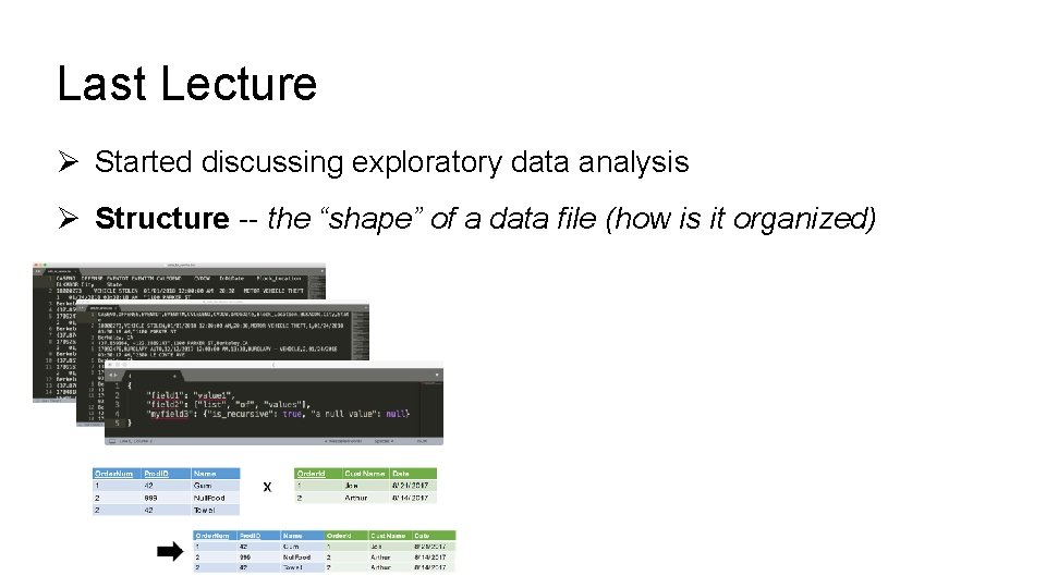
Last Lecture Ø Started discussing exploratory data analysis Ø Structure -- the “shape” of a data file (how is it organized)

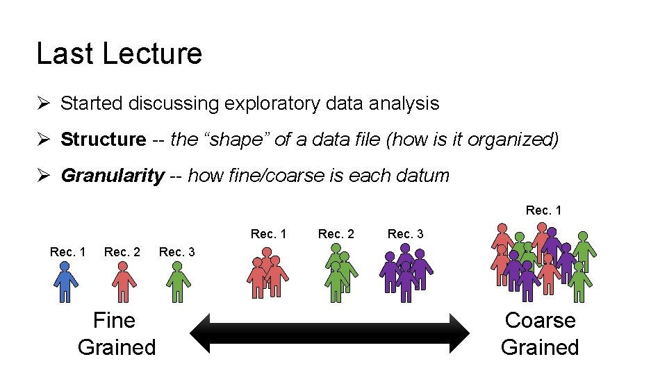
Last Lecture Ø Started discussing exploratory data analysis Ø Structure -- the “shape” of a data file (how is it organized) Ø Granularity -- how fine/coarse is each datum Rec. 1 Rec. 2 Fine Grained Rec. 2 Rec. 3 Coarse Grained

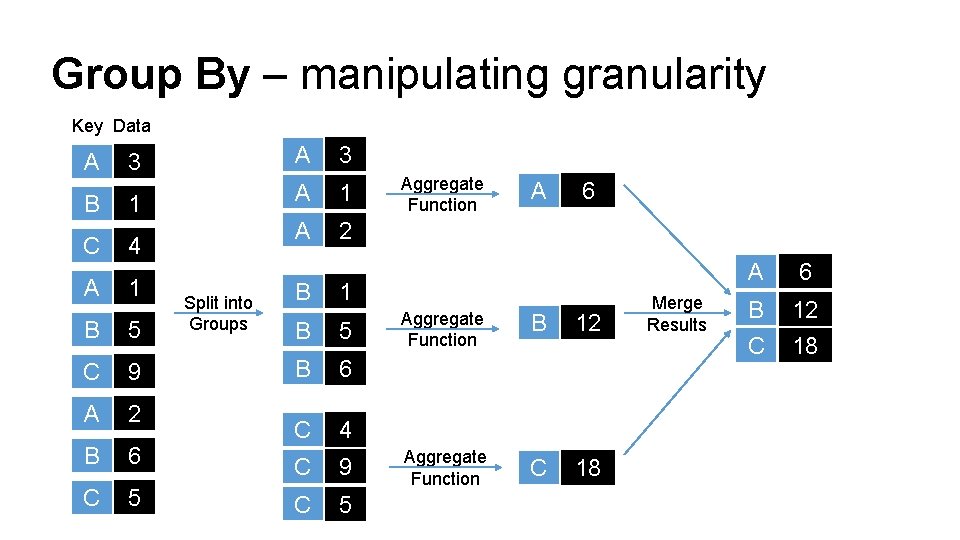
Group By – manipulating granularity Key Data 3 A 3 B 1 A 1 C 4 A 2 A 1 A B 5 C 9 A 2 B C Split into Groups B Aggregate Function A 6 1 B 5 B 6 6 C 4 C 9 5 C 5 Aggregate Function B 12 Aggregate Function C 18 Merge Results A 6 B 12 C 18

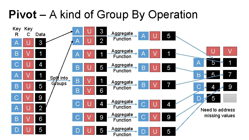
Pivot – A kind of Group By Operation Key R C Data A U 3 B V 1 C U 4 A V 1 B U 5 C V 9 A U 2 A U 3 A U 2 A B Split into Groups V U Aggregate Function A U 5 1 Aggregate Function A V 1 5 Aggregate Function B B V 1 B V 6 C U U V 5 7 4 Aggregate Function C U 4 C V 9 D U 5 B V 6 C V 9 Aggregate Function D U 5 Aggregate Function U V A 5 1 B 5 7 C 4 9 D 5 Need to address missing values

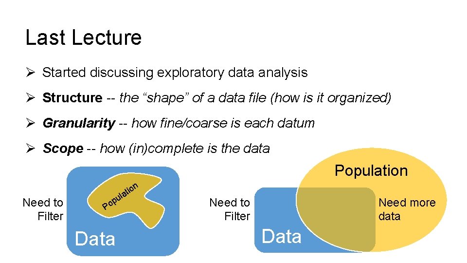
Last Lecture Ø Started discussing exploratory data analysis Ø Structure -- the “shape” of a data file (how is it organized) Ø Granularity -- how fine/coarse is each datum Ø Scope -- how (in)complete is the data Population n Need to Filter u io lat p o P Data Need to Filter Need more data Data

Last Lecture Ø Started discussing exploratory data analysis Ø Structure -- the “shape” of a data file (how is it organized) Ø Granularity -- how fine/coarse is each datum Ø Scope -- how (in)complete is the data Ø Temporality -- how is the data situated in time

Temporality Ø Data changes When was the data collected! Ø What is the meaning of a the time and date fields? Ø When the “event” happened? Ø When the data was collected or was entered into the system? Ø Date the data was copied into a database (look for many matching timestamps) Ø Time depends on where! (Time zones & daylight savings) Ø Learn to use datetime python library Ø Multiple string representation (depends on region): 07/08/09? Ø Are there strange null values? Ø January 1 st 1970, January 1 st 1900 Ø Is there periodicity? Diurnal patterns

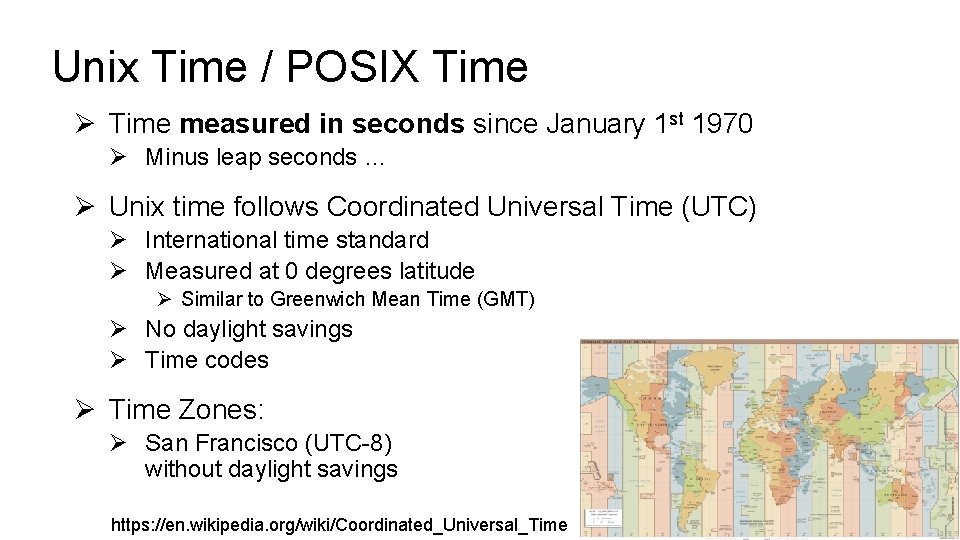
Unix Time / POSIX Time Ø Time measured in seconds since January 1 st 1970 Ø Minus leap seconds … Ø Unix time follows Coordinated Universal Time (UTC) Ø International time standard Ø Measured at 0 degrees latitude Ø Similar to Greenwich Mean Time (GMT) Ø No daylight savings Ø Time codes Ø Time Zones: Ø San Francisco (UTC-8) without daylight savings https: //en. wikipedia. org/wiki/Coordinated_Universal_Time

Key Data Properties to Consider in EDA Ø Structure -- the “shape” of a data file Ø Granularity -- how fine/coarse is each datum Ø Scope -- how (in)complete is the data Ø Temporality -- how is the data situated in time Ø Faithfulness -- how well does the data capture “reality”

Key Data Properties to Consider in EDA Ø Structure -- the “shape” of a data file Ø Granularity -- how fine/coarse is each datum Ø Scope -- how (in)complete is the data Ø Temporality -- how is the data situated in time Ø Faithfulness -- how well does the data capture “reality”

Faithfulness: Do I trust this data? Ø Does my data contain unrealistic or “incorrect” values? Ø Examples? Ø Ø Ø Dates in the future for events in the past Locations that don’t exist Negative counts Misspellings of names Large outliers Ø Does my data violate obvious dependencies? Ø E. g. , age and birthday don’t match Ø Was the data entered by hand? Ø Spelling errors, fields shifted … Ø Did the form require fields or provide default values? Ø Are there obvious signs of curb stoning (data falsification): Ø Repeated names, fake looking email addresses, repeated use of uncommon names or fields.

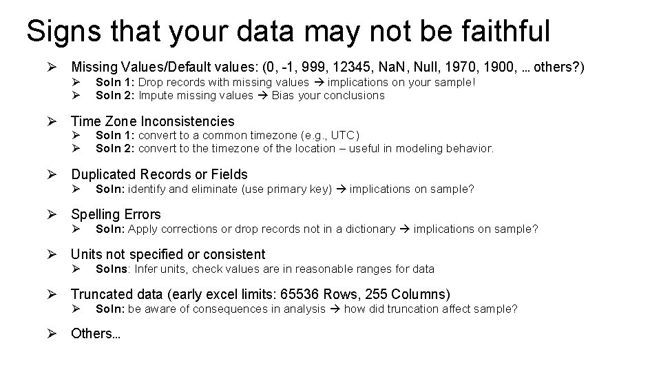
Signs that your data may not be faithful Ø Missing Values/Default values: (0, -1, 999, 12345, Na. N, Null, 1970, 1900, … others? ) Ø Ø Soln 1: Drop records with missing values implications on your sample! Soln 2: Impute missing values Bias your conclusions Ø Time Zone Inconsistencies Ø Ø Soln 1: convert to a common timezone (e. g. , UTC) Soln 2: convert to the timezone of the location – useful in modeling behavior. Ø Duplicated Records or Fields Ø Soln: identify and eliminate (use primary key) implications on sample? Ø Spelling Errors Ø Soln: Apply corrections or drop records not in a dictionary implications on sample? Ø Units not specified or consistent Ø Solns: Infer units, check values are in reasonable ranges for data Ø Truncated data (early excel limits: 65536 Rows, 255 Columns) Ø Soln: be aware of consequences in analysis how did truncation affect sample? Ø Others…

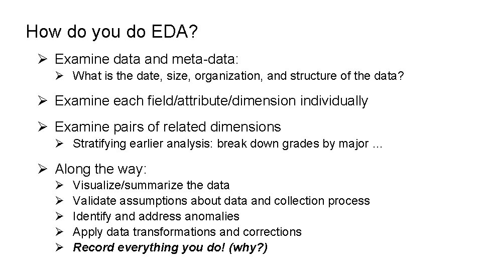
How do you do EDA? Ø Examine data and meta-data: Ø What is the date, size, organization, and structure of the data? Ø Examine each field/attribute/dimension individually Ø Examine pairs of related dimensions Ø Stratifying earlier analysis: break down grades by major … Ø Along the way: Ø Ø Ø Visualize/summarize the data Validate assumptions about data and collection process Identify and address anomalies Apply data transformations and corrections Record everything you do! (why? )

Visualization and EDA

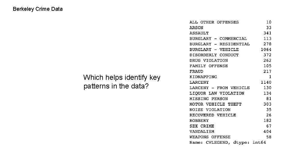
Berkeley Crime Data Which helps identify key patterns in the data?

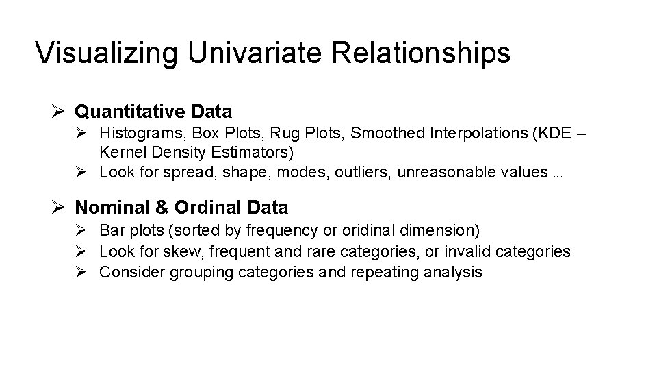
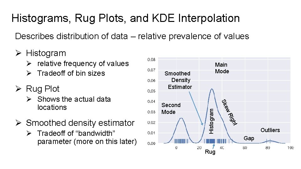
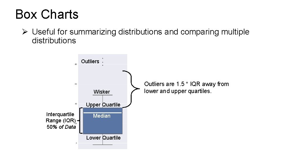
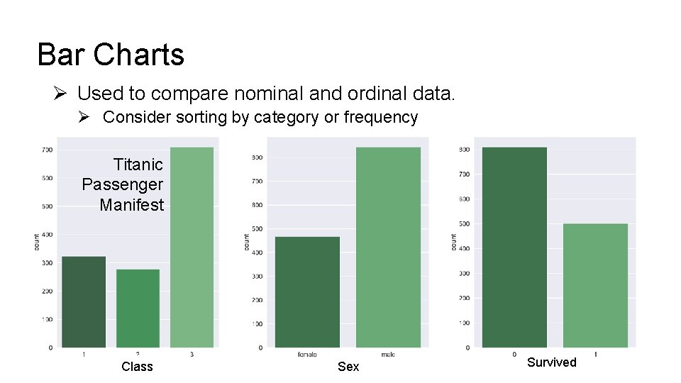
Visualizing Univariate Relationships Ø Quantitative Data Ø Histograms, Box Plots, Rug Plots, Smoothed Interpolations (KDE – Kernel Density Estimators) Ø Look for spread, shape, modes, outliers, unreasonable values … Ø Nominal & Ordinal Data Ø Bar plots (sorted by frequency or oridinal dimension) Ø Look for skew, frequent and rare categories, or invalid categories Ø Consider grouping categories and repeating analysis

Histograms, Rug Plots, and KDE Interpolation Describes distribution of data – relative prevalence of values Ø Histogram Ø Rug Plot ht Rig Ø Tradeoff of “bandwidth” parameter (more on this later) Second Mode ew Ø Smoothed density estimator Smoothed Density Estimator Sk Ø Shows the actual data locations Main Mode Histogram Ø relative frequency of values Ø Tradeoff of bin sizes Outliers Gap Rug

Box Charts Ø Useful for summarizing distributions and comparing multiple distributions Outliers Wisker Upper Quartile Interquartile Range (IQR) 50% of Data Median Lower Quartile Outliers are 1. 5 * IQR away from lower and upper quartiles.

Bar Charts Ø Used to compare nominal and ordinal data. Ø Consider sorting by category or frequency Titanic Passenger Manifest Class Sex Survived

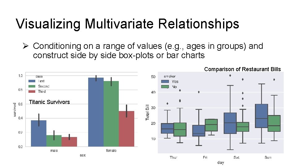
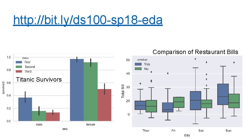
Visualizing Multivariate Relationships Ø Conditioning on a range of values (e. g. , ages in groups) and construct side by side box-plots or bar charts Comparison of Restaurant Bills Titanic Survivors

http: //bit. ly/ds 100 -sp 18 -eda Comparison of Restaurant Bills Titanic Survivors

Quick Break

Quick Break Scope: Do you have a full picture?

Berkeley Police Data Demo

Berkeley Police Public Datasets Ø Question: For this analysis we will not begin with a detailed question but instead a rough goal of understanding Police activity. Ø Examine Two Data Sets: Ø Call data Ø Stop data Ø Today we will work through the basic process of data loading, some preliminary cleaning, and exploratory data analysis.

Call Data Description Data pulled from Public Safety Server using data created for Berkeley’s Crime View Community page. Displays incidents reported for the last 180 days along with time, date, day of week and block level location information. The dataset reflects crimes as they have been reported to the BPD based on preliminary information supplied by the reporting parties. Preliminary crime classifications may change based on follow-up investigations. Not all calls for police service are included (e. g. Animal Bite). The information provided on this site is intended for use by the community to enhance their awareness of crimes occurring in their neighborhoods and the entire City. The data should not be used for in-depth crime analysis as the initial information is subject to change.

Stops Data Description This data was extracted from the Department’s Public Safety Server and covers the data beginning January 26, 2015. On January 26, 2015 the department began collecting data pursuant to General Order B-4 (issued December 31, 2014). Under that order, officers were required to provide certain data after making all vehicle detentions (including bicycles) and pedestrian detentions (up to five persons). This data set lists stops by police in the categories of traffic, suspicious vehicle, pedestrian and bicycle stops. Incident number, date and time, location and disposition codes are also listed in this data. Address data has been changed from a specific address, where applicable, and listed as the block where the incident occurred. Disposition codes were entered by officers who made the stop. These codes included the person(s) race, gender, age (range), reason for the stop, enforcement action taken, and whether or not a search was conducted.

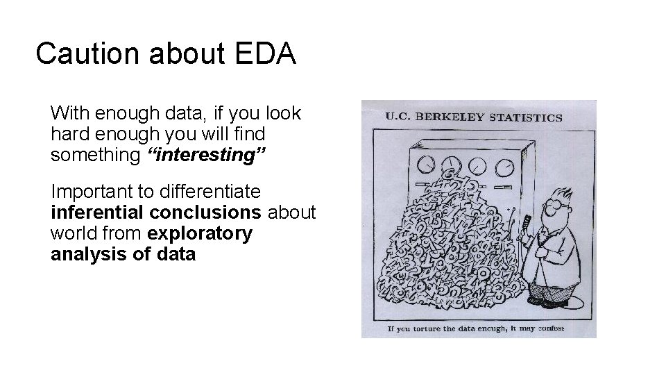
Caution about EDA With enough data, if you look hard enough you will find something “interesting” Important to differentiate inferential conclusions about world from exploratory analysis of data